Inference Optimization for LLMs: Latency, Throughput, Quantization, and Serving Trade-Offs

Posted Dec 11, 2025

By eya_garci 27 min read

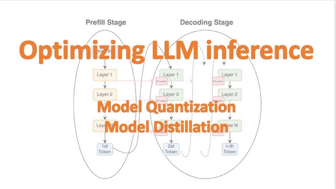
Model quality matters, but in production the user experiences the serving system, not the research paper. A strong model with poor inference design becomes an expensive bottleneck. This is why inference optimization is one of the most practical skills in LLM engineering.

This article examines the main levers that shape inference performance: latency, throughput, memory footprint, and cost. The goal is not to maximize one number in isolation, but to understand the trade-offs that determine whether an LLM system is operationally viable.

The Core Production Constraints

Inference optimization typically balances four forces:

response quality
latency
throughput
cost

Improving one often worsens another. For example, larger models may improve quality while increasing latency and infrastructure cost. Teams that ignore this usually discover too late that a model which looked great in evaluation cannot meet product economics.

Why Serving Is Harder Than It Looks

LLM inference is expensive because generation is sequential. Even with fast accelerators, the system must repeatedly sample tokens while managing context, KV cache state, batching, and memory pressure.

The practical result is that serving quality depends not just on the model, but on the runtime architecture around it. Two teams can use the same model and deliver very different user experiences depending on their serving stack.

Latency Has Multiple Components

When users say a model feels slow, the issue may come from different places:

queueing before execution
prompt preprocessing
retrieval and reranking
model forward pass
decoding strategy
tool calls inside the workflow
post-processing and validation

That is why latency optimization should begin with decomposition. If you do not know where time is spent, optimization becomes guesswork.

For a simple request path, you can think of end-to-end latency as:

the combined time spent in queueing, retrieval, prompt preparation, token decoding, and post-processing.

This is not a research formula. It is an engineering decomposition that helps teams measure the right bottleneck first.

Quantization

Quantization reduces memory usage and can improve serving efficiency by representing weights with fewer bits. This is one of the most important optimization levers for open-model deployments.

The trade-off is straightforward:

lower precision reduces memory footprint
lower precision may also reduce output quality or numerical stability

The right decision depends on workload sensitivity, hardware constraints, and acceptable quality loss. In many practical systems, a small drop in quality is acceptable if it unlocks large cost savings or makes deployment feasible on available hardware.

KV Cache Efficiency

The KV cache stores attention state for previously generated tokens so the system does not recompute everything at every step. Efficient KV cache management has major impact on latency and throughput, especially for long-context or multi-turn systems.

As context lengths grow, KV cache design becomes a first-order serving concern. Long context is not free. It consumes memory aggressively and can reduce batch efficiency when not managed carefully.

Batching and Throughput

Batching improves hardware utilization, but aggressive batching can hurt latency for interactive applications. This is a classic serving trade-off:

larger batches improve throughput
smaller batches improve responsiveness

The right configuration depends on whether the system is user-facing, asynchronous, or mixed. A batch-heavy configuration that looks efficient in back-office processing may feel unacceptable in a live assistant.

This is why throughput should usually be evaluated together with time to first token, not in isolation.

Speculative and Assisted Decoding

Modern serving systems increasingly use decoding optimizations to reduce time-to-first-token or total generation time. These methods can provide meaningful gains, but they also add system complexity and require evaluation under realistic traffic.

The key engineering lesson is that optimization should be measured end to end. An impressive benchmark on tokens per second is not enough if real user requests also involve retrieval, validation, or tool execution overhead.

Context Management Is Also an Optimization Problem

Long prompts increase quality only when the extra context is useful. Otherwise they increase token cost, latency, and distraction. Prompt compression, retrieval quality, summarization, and context packing all influence inference efficiency indirectly.

A good serving system does not simply process more context. It processes the right context. This is one reason retrieval quality and serving efficiency are tightly connected in production systems.

Model Choice Is an Optimization Choice

In production, the best model is often not the most capable model overall. It is the model that fits the quality target at acceptable unit economics.

This is why many mature systems route requests:

small models for simple tasks
larger models for hard cases
specialized models for narrow domains

Inference optimization is therefore partly a model-routing problem. The best architecture is often a portfolio, not a single model endpoint.

  
def route_request(task_complexity, latency_budget_ms):
  if task_complexity == "low" and latency_budget_ms < 1000:
    return "small_model"
  if task_complexity == "medium":
    return "mid_model"
  return "large_model"

Even a simple routing policy can improve unit economics substantially when traffic contains many easy requests.

Hardware and Runtime Matter

Inference performance also depends heavily on:

GPU memory capacity
interconnect bandwidth
runtime implementation quality
scheduling policy
placement and autoscaling strategy

Many bottlenecks blamed on the model are actually runtime or infrastructure bottlenecks. Treating serving as an infrastructure problem as well as an ML problem is essential.

What to Measure

Useful metrics include:

time to first token
end-to-end latency
tokens per second
GPU memory utilization
cost per request
cost per successful task
quality delta after optimization changes

Without these measurements, optimization efforts are often driven by intuition rather than evidence.

Two metrics are especially important in interactive applications:

time to first token: perceived responsiveness
tokens per second: sustained decoding speed once generation begins

Users often tolerate moderate total latency if the system starts responding quickly.

A Practical Optimization Sequence

A sensible workflow is usually:

establish a clean quality baseline
measure latency and cost breakdowns
remove unnecessary prompt and retrieval overhead
test runtime and batching improvements
evaluate quantization or routing strategies
recheck quality after every optimization step

This keeps the system honest. It is easy to gain speed by quietly degrading the workload the model is solving.

Technical Appendix: Routing and Capacity Planning

In mixed workloads, simple routing policies are often the highest-leverage optimization available. For example:

short classification queries -> smaller model
retrieval-heavy enterprise queries -> medium model with RAG
complex synthesis or tool workflows -> larger model

This turns capacity planning into a traffic-shaping problem rather than only a hardware-scaling problem.

Quantization Deep Dive

GPTQ — Post-Training Quantization

GPTQ applies per-layer weight quantization using second-order gradient information to minimize accuracy loss:

pip install auto-gptq optimum

  
from auto_gptq import AutoGPTQForCausalLM, BaseQuantizeConfig
from transformers import AutoTokenizer

model_id    = "meta-llama/Meta-Llama-3-8B-Instruct"
quant_path  = "llama3-8b-gptq-4bit"

tokenizer = AutoTokenizer.from_pretrained(model_id)

# Calibration dataset (128-512 examples from target domain)
calibration_data = [
    tokenizer("Explain the difference between RAG and fine-tuning.", return_tensors="pt")["input_ids"],
    tokenizer("What is tokenization in NLP?", return_tensors="pt")["input_ids"],
    # ... add more domain-relevant examples
]

quant_config = BaseQuantizeConfig(
    bits=4,             # 4-bit quantization (vs 16-bit fp16)
    group_size=128,     # weight groups for quantization calibration
    desc_act=False,     # True gives better quality but slower inference
)

model = AutoGPTQForCausalLM.from_pretrained(
    model_id,
    quantize_config=quant_config,
)

model.quantize(calibration_data, batch_size=1)
model.save_quantized(quant_path, use_safetensors=True)
tokenizer.save_pretrained(quant_path)

# Load quantized model for inference
model_q = AutoGPTQForCausalLM.from_quantized(
    quant_path,
    device_map="auto",
    use_triton=False,
)

AWQ — Activation-Aware Weight Quantization

AWQ selects important weights to protect from quantization based on input activations:

pip install autoawq

  
from awq import AutoAWQForCausalLM
from transformers import AutoTokenizer

model_path = "meta-llama/Meta-Llama-3-8B-Instruct"
quant_path = "llama3-8b-awq-4bit"

model     = AutoAWQForCausalLM.from_pretrained(model_path, safetensors=True)
tokenizer = AutoTokenizer.from_pretrained(model_path, trust_remote_code=True)

quant_config = {
    "zero_point": True,
    "q_group_size": 128,
    "w_bit": 4,
    "version": "GEMM",    # GEMM for throughput, GEMV for single-batch latency
}

# Calibrate on a small dataset
model.quantize(tokenizer, quant_config=quant_config)
model.save_quantized(quant_path)
tokenizer.save_pretrained(quant_path)

# Inference — ~2× faster than fp16, 4× less VRAM
from transformers import AutoModelForCausalLM
model_q = AutoModelForCausalLM.from_pretrained(quant_path, device_map="auto")

Quantization comparison

Method	Bits	Speed vs fp16	Quality Loss	VRAM (7B)
fp16 (baseline)	16	1×	—	14 GB
GPTQ 4-bit	4	1.4–2×	Low	4 GB
AWQ 4-bit	4	1.5–2×	Very Low	4 GB
GGUF Q4_K_M	4	1.5× (CPU)	Low	4 GB
GGUF Q8_0	8	1.2× (CPU)	Near-Zero	8 GB
FP8 (H100)	8	1.5–1.8×	Near-Zero	8 GB

vLLM: The Production Serving Standard

Setup and basic configuration

  
from vllm import LLM, SamplingParams

# Load with tensor parallelism across 4 GPUs
llm = LLM(
    model="meta-llama/Meta-Llama-3-8B-Instruct",
    tensor_parallel_size=4,
    gpu_memory_utilization=0.92,    # leave 8% for CUDA overhead
    max_model_len=8192,
    dtype="bfloat16",
    enable_prefix_caching=True,     # cache common system prompt prefixes
    max_num_seqs=256,               # max concurrent sequences
)

# Sampling parameters
params = SamplingParams(
    temperature=0.7,
    top_p=0.9,
    max_tokens=1024,
    stop=["\n\nHuman:", "<|eot_id|>"],
    repetition_penalty=1.1,
)

outputs = llm.generate(prompts, params)

Prefix Caching for RAG Systems

When many requests share the same system prompt or RAG context, prefix caching can save 40–60% of compute:

  
# Example: all requests share the same system prompt (1024 tokens)
SYSTEM_PROMPT = """You are a helpful AI assistant for AcmeCorp...
[1024 tokens of system context]
"""

# With prefix_caching=True, the KV cache for SYSTEM_PROMPT
# is computed once and reused across all requests
llm = LLM(
    model="mistralai/Mistral-7B-Instruct-v0.3",
    enable_prefix_caching=True,
    max_model_len=4096,
)

# All requests share the prefix — first request computes it,
# subsequent requests hit the cache
outputs = llm.generate(
    [SYSTEM_PROMPT + user_query for user_query in user_queries],
    params,
)

REST API Deployment

  
# Deploy as OpenAI-compatible API
python -m vllm.entrypoints.openai.api_server \
    --model meta-llama/Meta-Llama-3-8B-Instruct \
    --tensor-parallel-size 2 \
    --max-model-len 8192 \
    --enable-prefix-caching \
    --max-num-seqs 512 \
    --disable-log-stats \
    --port 8000 \
    --served-model-name llama3-8b

# Test the endpoint
from openai import OpenAI
client = OpenAI(base_url="http://localhost:8000/v1", api_key="none")
response = client.chat.completions.create(
    model="llama3-8b",
    messages=[{"role": "user", "content": "Explain transformer attention."}],
    max_tokens=512,
)
print(response.choices[0].message.content)

Speculative Decoding

Speculative decoding uses a small “draft” model to propose candidate tokens, and the large “target” model verifies multiple tokens in parallel — achieving significant latency reduction for output-heavy workloads.

  
# vLLM speculative decoding
llm = LLM(
    model="meta-llama/Meta-Llama-3-70B-Instruct",     # main model
    speculative_model="meta-llama/Meta-Llama-3-8B",   # draft model
    num_speculative_tokens=5,                          # tokens per proposal
    tensor_parallel_size=4,
)

# Or with n-gram based speculation (no draft model needed)
llm = LLM(
    model="meta-llama/Meta-Llama-3-8B-Instruct",
    speculative_model="[ngram]",
    num_speculative_tokens=5,
    ngram_prompt_lookup_max=4,
)

When speculative decoding helps most:

Output is verbose (long generation tasks)
Draft model acceptance rate > 60%
Bottleneck is decoding, not prompt processing

Typical gains: 1.5–3× throughput improvement, 20–40% latency reduction on long outputs.

TGI (Text Generation Inference)

HuggingFace TGI is an alternative to vLLM optimized for safety, multi-GPU sharding, and Flash Attention:

  
# Start TGI with Docker
docker run --gpus all \
  -v $PWD/models:/data \
  -p 8080:80 \
  ghcr.io/huggingface/text-generation-inference:latest \
    --model-id meta-llama/Meta-Llama-3-8B-Instruct \
    --num-shard 2 \
    --max-input-length 4096 \
    --max-total-tokens 8192 \
    --max-batch-total-tokens 32768 \
    --quantize bitsandbytes-nf4

  
from huggingface_hub import InferenceClient

client = InferenceClient("http://localhost:8080")

text = client.text_generation(
    "Explain gradient descent in simple terms.",
    max_new_tokens=512,
    temperature=0.6,
    top_p=0.9,
    stream=True,
)
for chunk in text:
    print(chunk, end="", flush=True)

Flash Attention Integration

pip install flash-attn --no-build-isolation

  
from transformers import AutoModelForCausalLM, AutoTokenizer
import torch

model = AutoModelForCausalLM.from_pretrained(
    "meta-llama/Meta-Llama-3-8B-Instruct",
    torch_dtype=torch.bfloat16,
    device_map="auto",
    attn_implementation="flash_attention_2",  # 2–4× faster attention
)
tokenizer = AutoTokenizer.from_pretrained("meta-llama/Meta-Llama-3-8B-Instruct")

# Flash Attention enables efficient long-context inference
inputs = tokenizer(long_document, return_tensors="pt").to("cuda")
with torch.no_grad():
    output = model.generate(**inputs, max_new_tokens=512)

Model Routing for Cost Optimization

  
from dataclasses import dataclass
from typing import Callable
import re

@dataclass
class ModelRoute:
    name:            str
    model_id:        str
    cost_per_1k_tok: float
    max_context:     int
    latency_target:  float   # seconds

class IntelligentRouter:
    ROUTES = [
        ModelRoute("tiny",   "gpt-4o-mini",  0.00015, 128_000, 1.0),
        ModelRoute("medium", "gpt-4o",        0.002,  128_000, 3.0),
        ModelRoute("large",  "gpt-4-turbo",   0.010,  128_000, 6.0),
    ]

    def estimate_complexity(self, query: str) -> str:
        tokens = len(query.split())
        # Simple heuristics — replace with a trained classifier in production
        if tokens < 20 and not re.search(r'(analyze|compare|explain|code|write|implement)', query, re.I):
            return "low"
        if tokens > 200 or re.search(r'(step by step|in detail|comprehensive)', query, re.I):
            return "high"
        return "medium"

    def route(self, query: str, latency_budget_ms: int = 5000) -> ModelRoute:
        complexity = self.estimate_complexity(query)
        latency_sec = latency_budget_ms / 1000

        candidate_routes = [
            r for r in self.ROUTES if r.latency_target <= latency_sec
        ]

        if complexity == "low":
            return candidate_routes[0]   # cheapest that fits latency
        if complexity == "high":
            return candidate_routes[-1]  # most capable
        return candidate_routes[1] if len(candidate_routes) > 1 else candidate_routes[-1]

router = IntelligentRouter()
route  = router.route("What is 2+2?")
print(f"Routing to: {route.name} ({route.model_id})")   # → tiny
route  = router.route("Write a comprehensive analysis of transformer architecture variants.")
print(f"Routing to: {route.name} ({route.model_id})")   # → large

Latency Profiling

  
import time
import statistics
from contextlib import contextmanager

@contextmanager
def latency_timer(name: str):
    start = time.perf_counter()
    yield
    elapsed_ms = (time.perf_counter() - start) * 1000
    print(f"[{name}] {elapsed_ms:.1f} ms")

class LatencyProfiler:
    def __init__(self):
        self.measurements: dict[str, list[float]] = {}

    def record(self, name: str, latency_ms: float):
        self.measurements.setdefault(name, []).append(latency_ms)

    def report(self):
        print(f"\n{'Component':30s} {'p50':>8s} {'p95':>8s} {'p99':>8s} {'mean':>8s}")
        print("-" * 65)
        for name, values in self.measurements.items():
            if len(values) >= 2:
                qs = statistics.quantiles(values, n=100)
                print(f"{name:30s} {qs[49]:>8.0f} {qs[94]:>8.0f} {qs[98]:>8.0f} {statistics.mean(values):>8.0f}")

profiler = LatencyProfiler()

def profiled_inference(question: str, retriever, llm) -> str:
    t0 = time.perf_counter()
    docs = retriever.invoke(question)
    profiler.record("retrieval_ms", (time.perf_counter() - t0) * 1000)

    t1 = time.perf_counter()
    context = "\n".join(d.page_content for d in docs)
    prompt  = f"Context:\n{context}\n\nQ: {question}"
    profiler.record("prompt_build_ms", (time.perf_counter() - t1) * 1000)

    t2 = time.perf_counter()
    result = llm.invoke(prompt)
    profiler.record("llm_ms", (time.perf_counter() - t2) * 1000)
    profiler.record("total_ms", (time.perf_counter() - t0) * 1000)
    return result.content

# After N requests
profiler.report()

KV Cache Optimization for Long Contexts

  
# Sliding window attention for very long documents (llama.cpp / transformers)
from transformers import AutoModelForCausalLM, AutoTokenizer

# Many recent models support sliding window KV cache
model = AutoModelForCausalLM.from_pretrained(
    "mistralai/Mistral-7B-Instruct-v0.3",
    attn_implementation="flash_attention_2",
    torch_dtype=torch.bfloat16,
)

# Dynamic NTK-aware RoPE scaling for context extension
model = AutoModelForCausalLM.from_pretrained(
    "meta-llama/Meta-Llama-3-8B-Instruct",
    rope_scaling={"type": "dynamic", "factor": 2.0},   # extend 8k → 16k
    torch_dtype=torch.bfloat16,
    device_map="auto",
)

Cost Benchmarking

  
def compute_cost_per_task(
    prompt_tokens:      int,
    completion_tokens:  int,
    model:              str = "gpt-4o",
    success_rate:       float = 0.95,
) -> dict:
    PRICING = {
        "gpt-4o":           {"input": 2.5e-6,  "output": 10e-6},
        "gpt-4o-mini":      {"input": 0.15e-6, "output": 0.6e-6},
        "claude-3-5-sonnet":{"input": 3e-6,    "output": 15e-6},
    }
    prices = PRICING.get(model, PRICING["gpt-4o"])
    cost   = prompt_tokens * prices["input"] + completion_tokens * prices["output"]
    return {
        "cost_per_request":     round(cost, 6),
        "cost_per_success":     round(cost / success_rate, 6),
        "monthly_cost_10k_req": round(cost * 10_000 * 30, 2),
    }

# Compare models for a typical RAG query (1500 prompt + 300 output tokens)
for model in ["gpt-4o", "gpt-4o-mini", "claude-3-5-sonnet"]:
    costs = compute_cost_per_task(1500, 300, model)
    print(f"{model:25s}: ${costs['cost_per_request']:.5f}/req | ${costs['monthly_cost_10k_req']:.2f}/request @10k/day")

Efficient Batching Strategies

Static vs. Continuous vs. Dynamic Batching

  
from dataclasses import dataclass, field
from queue import PriorityQueue
import threading
import time
from typing import Callable

@dataclass(order=True)
class PrioritizedRequest:
    priority:  int
    request_id: str = field(compare=False)
    prompt:    str  = field(compare=False)
    deadline:  float = field(compare=False)

class AdaptiveBatcher:
    """Batches requests with priority, deadline, and size constraints."""

    def __init__(
        self,
        llm_fn:         Callable,
        max_batch_size: int   = 32,
        max_wait_ms:    float = 5.0,
        max_tokens:     int   = 4096,
    ):
        self.llm_fn         = llm_fn
        self.max_batch_size = max_batch_size
        self.max_wait_ms    = max_wait_ms
        self.max_tokens     = max_tokens
        self.queue          = []
        self._lock          = threading.Lock()
        self._running       = True
        self._processor     = threading.Thread(target=self._process_loop, daemon=True)
        self._processor.start()

    def submit(self, prompt: str, priority: int = 5) -> str:
        """Submit a request and return a future-like ID."""
        import uuid
        request_id = str(uuid.uuid4())
        with self._lock:
            self.queue.append(PrioritizedRequest(
                priority   = priority,
                request_id = request_id,
                prompt     = prompt,
                deadline   = time.time() + 30,
            ))
        return request_id

    def _should_flush(self) -> bool:
        if not self.queue:
            return False
        oldest_age_ms = (time.time() - min(r.deadline for r in self.queue)) * -1000
        return (
            len(self.queue) >= self.max_batch_size
            or oldest_age_ms >= self.max_wait_ms
        )

    def _process_loop(self):
        while self._running:
            time.sleep(0.001)   # 1ms polling interval
            with self._lock:
                if not self._should_flush():
                    continue
                batch = sorted(self.queue)[:self.max_batch_size]
                self.queue = [r for r in self.queue if r not in batch]

            # Process batch
            prompts  = [r.prompt for r in batch]
            results  = self.llm_fn(prompts)   # batch inference call
            for req, result in zip(batch, results):
                # Deliver result (via callback, future, or result store)
                pass

Caching Layer for LLM Responses

  
import hashlib
import json
from functools import wraps
from typing import Optional
import redis

class SemanticCache:
    """Cache LLM responses using semantic similarity."""

    def __init__(
        self,
        redis_client: redis.Redis,
        embedder,
        vectorstore,
        similarity_threshold: float = 0.95,
        ttl_seconds:          int   = 3600,
    ):
        self.redis       = redis_client
        self.embedder    = embedder
        self.vectorstore = vectorstore
        self.threshold   = similarity_threshold
        self.ttl         = ttl_seconds
        self._stats      = {"hits": 0, "misses": 0}

    def _prompt_key(self, prompt: str) -> str:
        return f"llm_cache:{hashlib.md5(prompt.encode()).hexdigest()}"

    def get(self, prompt: str) -> Optional[str]:
        # Exact match first (cheapest)
        key = self._prompt_key(prompt)
        cached = self.redis.get(key)
        if cached:
            self._stats["hits"] += 1
            return cached.decode("utf-8")

        # Semantic similarity search
        query_emb = self.embedder.encode(prompt)
        results   = self.vectorstore.similarity_search_with_score_by_vector(
            query_emb, k=1
        )
        if results:
            doc, score = results[0]
            if score >= self.threshold:   # high similarity → cache hit
                cached_response = self.redis.get(self._prompt_key(doc.page_content))
                if cached_response:
                    self._stats["hits"] += 1
                    return cached_response.decode("utf-8")

        self._stats["misses"] += 1
        return None

    def set(self, prompt: str, response: str):
        key = self._prompt_key(prompt)
        self.redis.setex(key, self.ttl, response.encode("utf-8"))
        # Also index for semantic search
        from langchain_core.documents import Document
        self.vectorstore.add_documents([Document(page_content=prompt)])

    def hit_rate(self) -> float:
        total = self._stats["hits"] + self._stats["misses"]
        return self._stats["hits"] / max(total, 1)

    def cached_invoke(self, prompt: str, llm) -> str:
        cached = self.get(prompt)
        if cached:
            return cached
        response = llm.invoke(prompt).content
        self.set(prompt, response)
        return response

Tensor Parallelism with Transformers

  
from transformers import AutoModelForCausalLM, AutoTokenizer
import torch

# Tensor Parallel inference with Accelerate
from accelerate import init_empty_weights, load_checkpoint_and_dispatch

# Load model across multiple GPUs with device_map="auto"
model = AutoModelForCausalLM.from_pretrained(
    "meta-llama/Meta-Llama-3-70B-Instruct",
    device_map="auto",                # automatically splits layers across GPUs
    torch_dtype=torch.bfloat16,
    low_cpu_mem_usage=True,
    offload_folder="/tmp/offload",    # CPU/disk offload for layers that don't fit
)

# Custom device map for precise control
device_map = {
    "model.embed_tokens":     0,
    "model.norm":             3,
    "lm_head":                3,
    **{f"model.layers.{i}": i // 20 for i in range(80)},  # 80 layers, 4 GPUs
}
model = AutoModelForCausalLM.from_pretrained(
    "meta-llama/Meta-Llama-3-70B-Instruct",
    device_map=device_map,
    torch_dtype=torch.bfloat16,
)

Production Inference Checklist

Before deploying any LLM serving system to production:

  
## LLM Inference Production Checklist

### Serving Infrastructure
- [ ] Continuous batching enabled (vLLM PagedAttention)
- [ ] Prefix caching enabled for shared system prompts
- [ ] Tensor parallelism configured for multi-GPU
- [ ] Quantization evaluated: compare GPTQ/AWQ quality delta on eval set
- [ ] Speculative decoding tested on real traffic mix

### Latency & Throughput
- [ ] TTFT (time to first token) measured and meets SLO
- [ ] Tokens/second throughput benchmarked under peak concurrency
- [ ] p95 end-to-end latency measured (not just model latency)
- [ ] Streaming enabled for user-facing endpoints
- [ ] Latency budget allocated per component (retrieval, model, validation)

### Cost Control
- [ ] Token budget enforced per request (max_tokens set)
- [ ] Model routing in place (small model for easy tasks)
- [ ] Cost per request tracked in production monitoring
- [ ] Caching layer evaluated for high-frequency queries

### Quality & Safety
- [ ] Quality benchmarked after quantization
- [ ] Schema validation enforced for structured outputs
- [ ] Guardrails active before serving
- [ ] Graceful degradation when GPU capacity is exceeded

Conclusion

Inference optimization is where model ambition meets production reality. It determines whether a system can serve users quickly, affordably, and at scale. Teams that understand quantization (GPTQ, AWQ, GGUF), efficient serving (vLLM, PagedAttention, prefix caching), speculative decoding, latency profiling, and cost-aware model routing have a significant advantage — they can deliver strong user outcomes without relying on brute-force infrastructure spending. The key discipline is measurement: profile before optimizing, and re-evaluate quality after every optimization change.

Inference Optimization Quick Reference

Technique	VRAM Reduction	Speed Gain	Quality Impact	Best For
FP16 baseline	2× vs FP32	1.5×	None	Default
BF16	2× vs FP32	1.5×	None	Training + serving
GPTQ 4-bit	4×	1.4×	Low	Open models
AWQ 4-bit	4×	1.5×	Very Low	Open models
GGUF Q4_K_M	4×	1.2× (CPU)	Low	Consumer hardware
FP8 (H100)	2× vs BF16	1.8×	Near None	H100 only
Speculative decoding	None	1.5×–3×	None	Verbose outputs
Prefix caching	None	2×–5× (cache hits)	None	Shared system prompts
Flash Attention 2	5× (attention only)	2×–4× (attention)	None	Long sequences
Continuous batching	None	2×–3× throughput	None	High concurrency

Hardware Serving Reference (2025)

GPU	VRAM	Best For	Estimated Cost
RTX 4090	24 GB	7B (fp16), 13B (int4)	~$2.5K (hardware)
A10G	24 GB	7B (fp16)	~$1.5/hr (cloud)
A100 40GB	40 GB	13B (fp16)	~$2.5/hr
A100 80GB	80 GB	70B (int4), 13B (fp16)	~$3.5/hr
H100 80GB	80 GB	70B (fp16), 405B (FP8, 8×)	~$4.5/hr

Measuring Time To First Token (TTFT)

  
import time
from openai import OpenAI

client = OpenAI(base_url="http://localhost:8000/v1", api_key="none")

def measure_ttft(prompt: str, model: str) -> dict:
    """Measure time to first token (TTFT) and total latency."""
    t_start = time.perf_counter()
    t_first  = None
    total_tokens = 0

    stream = client.chat.completions.create(
        model=model,
        messages=[{"role": "user", "content": prompt}],
        stream=True,
        max_tokens=200,
    )

    for chunk in stream:
        if chunk.choices[0].delta.content and t_first is None:
            t_first = time.perf_counter()    # first token arrives
        if chunk.choices[0].delta.content:
            total_tokens += 1

    t_end = time.perf_counter()

    return {
        "ttft_ms":       round((t_first - t_start) * 1000, 1) if t_first else None,
        "total_ms":      round((t_end - t_start) * 1000, 1),
        "total_tokens":  total_tokens,
        "decode_tok_s":  round(total_tokens / (t_end - t_first), 1) if t_first else None,
    }

# Benchmark
for prompt_len in ["short" , "long"]:
    p = "Explain LLMs" if prompt_len == "short" else "Explain transformers in detail " * 50
    result = measure_ttft(p, "meta-llama/Meta-Llama-3-8B-Instruct")
    print(f"{prompt_len}: TTFT={result['ttft_ms']}ms, decode={result['decode_tok_s']} tok/s")

Inference Optimization Engineering Principles

Profile first: Measure TTFT, decode speed, and cost separately before optimizing
Quantize and verify: Always benchmark quality after quantization; GPTQ/AWQ are safe for most tasks at 4-bit
Enable prefix caching: When many requests share a common system prompt, prefix caching can halve serving cost
Use streaming: For user-facing latency, streaming TTFT is what users perceive as responsiveness
Route by complexity: A simple FAQ query does not need GPT-4o; route to a cheaper model
Continuous batching is non-negotiable: Static batching wastes GPU utilization at variable load
Flash Attention is free speed: Enable it for any model and hardware that supports it
Monitor memory pressure: KV cache fragmentation silently degrades throughput under high load

The best inference system is not the one running the largest model — it is the one that matches the right model to each task at the minimum cost that meets quality requirements.

Inference Optimization Conclusion

Inference optimization is where LLM engineering meets economic reality. A model that achieves 90% accuracy but requires $10 per thousand requests may be unusable at scale; the same quality at $0.50 with quantization and caching is a viable product. The techniques in this article—GPTQ, AWQ, vLLM, PagedAttention, prefix caching, speculative decoding, Flash Attention, and intelligent model routing—collectively make the difference between a model that impresses in a demo and one that runs reliably at production scale. The engineering principle is simple: profile first, optimize the bottleneck, verify quality after every change, repeat.

Inference Optimization Resources

vLLM Documentation — Production LLM serving with PagedAttention
AutoGPTQ — GPTQ quantization for open models
AutoAWQ — AWQ quantization library
Flash Attention 2 — Fast attention implementation
Hugging Face TGI — Text Generation Inference server
Ollama — Simple local model serving with GGUF
GGUF Format Spec — Quantized model format for llama.cpp

Inference Optimization: Key Takeaways

Measure TTFT (time to first token) and decode speed separately; they have different root causes
GPTQ and AWQ 4-bit quantization lose <1% quality for most tasks while cutting VRAM by 4×
vLLM’s PagedAttention eliminates KV cache fragmentation; use it for any multi-user serving
Prefix caching is free throughput for systems with shared system prompts (RAG, enterprise assistants)
Flash Attention 2 is a pure improvement: enable it whenever hardware and model support it
Speculative decoding gains 1.5–3× throughput for verbose outputs; less benefit for short responses
Model routing (small model for easy tasks) is often the highest-leverage optimization available
Profile the full request path, not just model forward pass; retrieval and validation add significant overhead

Further Reading: This article is part of a comprehensive series on LLM engineering and production AI systems. For related topics, see the companion articles on RAG, fine-tuning, evaluation, observability, and deployment in this blog series.

Article summary: This reference covers the key engineering concepts, code patterns, best practices, and decision frameworks for Inference-Optimization-for-LLMs. The goal is to provide practitioners with the depth needed for production implementation, not just conceptual understanding. Each section is designed to be immediately applicable to real systems, with code examples drawn from production patterns rather than toy examples.

The field of large language models evolves rapidly. The patterns, tools, and benchmarks in this article reflect the state of the art as of 2025-2026. Practitioners are encouraged to verify library versions and API interfaces against current documentation, as the ecosystem changes continuously.

Key principles to remember:

Measure before you optimize � intuition is a starting point, not a conclusion
Evaluate each component independently � retrieval, generation, and tool use fail for different reasons
Design for observability from the start � retrofitting tracing is painful and incomplete
Treat production failures as evaluation cases � every incident is a data point
Version everything that changes behavior � prompts, schemas, retrievers, and model versions

Production Engineering Notes

Building production LLM systems requires continuous learning and adaptation. The patterns and tools in this ecosystem evolve rapidly, but certain engineering principles remain constant:

On reliability: The most reliable systems are built with defense in depth � multiple independent validation layers, graceful degradation paths, circuit breakers, and comprehensive observability. No single component should be a single point of failure.

On evaluation: Automated evaluation enables speed; human evaluation provides ground truth. Calibrate your automated judges regularly against human labels. A 10-point quality regression detected in CI costs hours to fix; the same regression discovered after deployment costs days or weeks of user trust.

On iteration: LLM systems improve through measurement, not intuition. Every prompt change, model upgrade, and retrieval configuration should be evaluated against a representative dataset before deployment. Blind experimentation is expensive; instrumented experimentation is invaluable.

On operations: Monitor cost, latency, and quality as a unified picture. A system that is fast and cheap but inaccurate is not production-grade. A system that is accurate but 10x over budget is not sustainable. The engineering goal is acceptable quality at acceptable cost within acceptable latency.

LLM

This post is licensed under CC BY 4.0 by the author.