Mixture of Experts: Architecture, Training, and Production Trade-Offs

Posted Dec 14, 2025

By eya_garci 31 min read

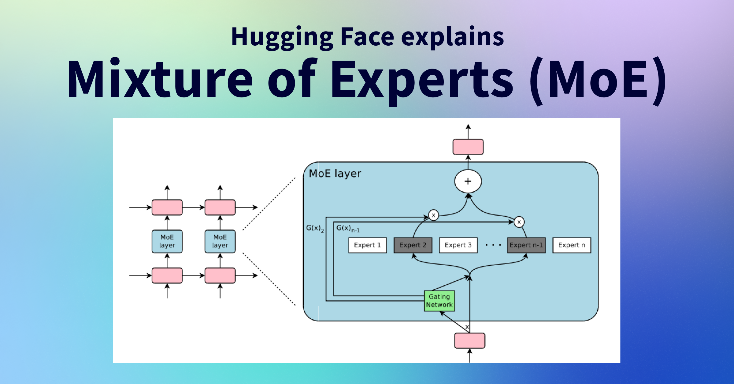
Mixture of Experts (MoE) is one of the most important architectural ideas behind the largest and most efficient modern language models. It enables scaling model capacity without proportionally increasing compute cost. Models like Mixtral 8x7B, GPT-4 (reportedly), and Switch Transformer are built on MoE principles. Yet MoE models also introduce unique training instabilities and serving challenges that pure dense models do not have.

This article explains how MoE works, why it matters, and what engineering trade-offs it introduces.

The Core Problem MoE Solves

Dense transformer models activate every parameter for every input token. A 70B parameter model uses all 70B parameters to process every token. This is computationally expensive and scales quadratically in terms of memory access.

MoE decouples model capacity (total parameter count) from compute cost (parameters activated per token). In an MoE model, different tokens are routed to different subsets of the network — called experts. Each token only activates a fraction of the total parameters.

The result: a 47B parameter Mixtral 8x7B model uses approximately 13B active parameters per token — comparable in compute to a 13B dense model, but with the representational capacity of a much larger network.

Architecture

An MoE model replaces the feed-forward network (FFN) in each transformer block with a mixture of expert FFNs and a router.

Standard transformer block (dense)

Input → Layer Norm → Attention → Residual → Layer Norm → FFN → Residual → Output

MoE transformer block

Input → Layer Norm → Attention → Residual → Layer Norm → [Router + Expert Pool] → Residual → Output

The MoE layer contains:

N expert networks: each a standard FFN with its own weights
A router (gating network): a small linear layer that produces a probability distribution over experts for each token

Top-K routing

For each token, the router selects the top-K experts by probability and routes the token to only those experts. K=1 (hard routing) or K=2 (soft routing) are the most common choices.

\[y = \sum_{i \in \text{Top-K}(G(x))} G(x)_i \cdot E_i(x)\]

where $G(x)$ is the router output (softmax over experts), $E_i(x)$ is the output of expert $i$, and Top-K selects the K highest-probability experts.

The final output is a weighted sum of the selected experts’ outputs.

  
import torch
import torch.nn as nn
import torch.nn.functional as F

class MoELayer(nn.Module):
    def __init__(self, d_model, d_ff, num_experts=8, top_k=2):
        super().__init__()
        self.num_experts = num_experts
        self.top_k = top_k
        self.router = nn.Linear(d_model, num_experts, bias=False)
        self.experts = nn.ModuleList([
            nn.Sequential(
                nn.Linear(d_model, d_ff),
                nn.SiLU(),
                nn.Linear(d_ff, d_model)
            )
            for _ in range(num_experts)
        ])

    def forward(self, x):
        # x: [batch, seq_len, d_model]
        B, T, D = x.shape
        x_flat = x.view(B * T, D)

        router_logits = self.router(x_flat)              # [B*T, num_experts]
        router_probs = F.softmax(router_logits, dim=-1)

        topk_probs, topk_indices = router_probs.topk(self.top_k, dim=-1)
        topk_probs = topk_probs / topk_probs.sum(dim=-1, keepdim=True)  # renormalize

        output = torch.zeros_like(x_flat)
        for k in range(self.top_k):
            expert_indices = topk_indices[:, k]
            expert_weights = topk_probs[:, k].unsqueeze(-1)
            for e in range(self.num_experts):
                mask = (expert_indices == e)
                if mask.any():
                    output[mask] += expert_weights[mask] * self.experts[e](x_flat[mask])

        return output.view(B, T, D)

The Load Balancing Problem

Naively trained MoE models suffer from expert collapse: the router consistently routes all tokens to a small number of experts, leaving the rest idle. This wastes parameters and causes uneven compute load during distributed training.

Auxiliary load balancing loss

Add a differentiable loss term that penalizes imbalanced routing:

\[\mathcal{L}_{\text{balance}} = \alpha \cdot N \cdot \sum_{i=1}^{N} f_i \cdot P_i\]

where $f_i$ is the fraction of tokens routed to expert $i$, $P_i$ is the average router probability for expert $i$, and $\alpha$ is a coefficient (typically 0.01 to 0.001).

  
def load_balancing_loss(router_probs, topk_indices, num_experts, alpha=0.01):
    # router_probs: [num_tokens, num_experts]
    # topk_indices: [num_tokens, top_k]
    num_tokens = router_probs.shape[0]
    
    # fraction of tokens per expert
    expert_mask = F.one_hot(topk_indices, num_experts).float().sum(dim=1)
    f = expert_mask.mean(dim=0)  # [num_experts]
    
    # mean router probability per expert
    P = router_probs.mean(dim=0)  # [num_experts]
    
    return alpha * num_experts * (f * P).sum()

Expert capacity

In distributed training, each expert runs on a specific device. To prevent some devices from being overwhelmed, a capacity factor limits how many tokens a single expert processes per batch. Tokens that exceed this limit are dropped or handled by a fallback expert.

Key MoE Variants

Switch Transformer (Google, 2021)

Used top-1 routing (each token goes to exactly one expert). Demonstrated that even hard routing stabilizes with the right auxiliary loss. Scaled to 1.6 trillion parameters on 2048 TPU cores.

GLaM (Google, 2021)

64 experts per layer, top-2 routing. Matched GPT-3 quality with 1/3 the energy cost during training.

Mixtral 8x7B (Mistral AI, 2023)

8 experts per MoE layer, top-2 routing. Dense layers otherwise (attention is shared). 47B total parameters, ~13B active. Outperformed LLaMA 2 70B on most benchmarks.

DeepSeek-V2 (2024)

Fine-grained experts (160 experts, top-6 routing). Introduced multi-head latent attention + MoE. Demonstrated that increasing expert count while keeping active parameters fixed improves performance.

Training MoE Models

MoE training is harder than dense model training. Key issues:

Communication overhead

In data-parallel distributed training, each expert receives tokens from all ranks. This requires all-to-all communication — every device sends tokens to every other device. This is expensive at scale.

Gradient instability

Router logits can become very large early in training, causing unstable routing decisions. Fixes include router z-loss (penalizing large logits) and careful initialization.

\[\mathcal{L}_z = \frac{\beta}{N} \sum_{i=1}^{N} \left(\log \sum_{j=1}^{N} e^{x_i^{(j)}}\right)^2\]

Expert specialization

Over time, experts tend to specialize on different types of tokens or linguistic patterns. This specialization is desirable but takes many training steps to emerge. Early training with strong load balancing loss is important.

Inference and Serving Challenges

MoE models have a different operational profile from dense models.

Memory requirements

All expert weights must be loaded into memory even though only K of them are used per token. A Mixtral 8x7B model requires loading all 47B parameters, while only 13B are active per forward pass. This means:

Memory: scales with total parameters (same as a 47B dense model)
Compute: scales with active parameters (~13B per token)

Expert parallelism

For efficient serving, each expert is placed on a dedicated GPU (or set of GPUs). This requires expert parallelism in addition to tensor and pipeline parallelism. Frameworks like Megablocks and vLLM support MoE-specific serving strategies.

Latency vs. throughput tradeoff

MoE models excel at throughput (many requests batched together, activating diverse experts in parallel) but can have higher latency for single-request inference because all tokens still need routing decisions.

Quantization effects

Quantizing MoE models is more complex. Experts have different weight distributions, so per-expert calibration is needed. GPTQ and AWQ both support MoE quantization.

When to Use MoE

Scenario	Use MoE?
Training budget fixed, want max capacity	Yes — same FLOPs, larger model
Inference on single GPU, memory is tight	Careful — full parameter load required
High-throughput multi-user serving	Yes — experts activate in parallel across batch
Single-user interactive latency-critical	Dense model may have lower p50 latency
Domain diversity in corpus	Yes — experts naturally specialize
Fine-tuning a pretrained MoE	Yes — LoRA adapters work per-expert

MoE + LoRA Fine-Tuning

Fine-tuning a Mixtral-style MoE with LoRA applies rank-decomposed adapters to each expert independently:

  
from peft import LoraConfig, get_peft_model
from transformers import AutoModelForCausalLM

model = AutoModelForCausalLM.from_pretrained("mistralai/Mixtral-8x7B-v0.1")

lora_config = LoraConfig(
    r=16,
    lora_alpha=32,
    target_modules=["q_proj", "v_proj", "w1", "w2", "w3"],  # include expert FFN layers
    lora_dropout=0.05,
    bias="none",
    task_type="CAUSAL_LM",
)

model = get_peft_model(model, lora_config)
model.print_trainable_parameters()
# trainable params: ~50M | all params: ~47B | trainable: 0.1%

Summary: MoE vs Dense Trade-Offs

Dimension	Dense	MoE
Memory (inference)	Scales with active params	Scales with total params
Compute per token	High (all params)	Low (K/N fraction)
Training stability	High	Moderate — needs load balancing
Serving complexity	Simple	Requires expert parallelism
Specialization	None	Natural expert specialization
Throughput efficiency	Linear	Super-linear at high batch size
Peak capability at fixed FLOPs	Lower	Higher

Expert Analysis: Expert Specializations

Research on trained MoE models reveals that experts develop soft specializations:

Syntactic experts: Handle tokens related to punctuation, function words, and grammar structure
Semantic domain experts: Activate more for technical vs. general language
Language-specific experts: Multilingual MoE models develop cross-lingual and language-specific specialists
Format experts: Specialize in code, prose, numbers, or structured data

These specializations emerge without explicit supervision — the router learns them through end-to-end training.

Inspecting expert utilization

  
import torch
import torch.nn.functional as F
from collections import defaultdict

class ExpertAnalyzer:
    """Hook-based expert utilization tracker."""

    def __init__(self, model, layer_indices: list[int]):
        self.model      = model
        self.layer_ids  = layer_indices
        self.activations = defaultdict(list)
        self._hooks     = []
        self._register_hooks()

    def _register_hooks(self):
        for layer_id in self.layer_ids:
            layer = self.model.model.layers[layer_id].mlp
            hook  = layer.gate.register_forward_hook(
                lambda m, inp, out, lid=layer_id: self._capture(lid, out)
            )
            self._hooks.append(hook)

    def _capture(self, layer_id: int, gate_output: torch.Tensor):
        # gate_output: [batch * seq_len, num_experts]
        topk_indices = gate_output.topk(2, dim=-1).indices   # top-2
        self.activations[layer_id].append(topk_indices.cpu())

    def compute_utilization(self, num_experts: int = 8) -> dict[int, torch.Tensor]:
        result = {}
        for layer_id, act_list in self.activations.items():
            all_indices = torch.cat(act_list, dim=0)   # [N, top_k]
            counts      = torch.zeros(num_experts)
            for idx in all_indices.flatten():
                counts[idx.item()] += 1
            result[layer_id] = counts / counts.sum()
        return result

    def print_utilization_report(self, num_experts: int = 8):
        utilization = self.compute_utilization(num_experts)
        for layer_id, dist in utilization.items():
            print(f"\nLayer {layer_id} expert utilization:")
            for i, p in enumerate(dist):
                bar = "█" * int(p * 50)
                print(f"  Expert {i}: {p:.3f} {bar}")

    def remove_hooks(self):
        for hook in self._hooks:
            hook.remove()

# Usage
analyzer = ExpertAnalyzer(model, layer_indices=[0, 8, 16, 24])
with torch.no_grad():
    for batch in eval_dataloader:
        model(**batch)
analyzer.print_utilization_report()
analyzer.remove_hooks()

Expert Parallelism for Inference

For production serving of large MoE models, expert parallelism places different experts on different GPU ranks:

  
# Conceptual expert-parallel serving layout
# Mixtral 8x7B with 8 experts, 8 GPUs

# Each GPU hosts 1 expert per MoE layer
# GPU 0: Expert 0 for all MoE layers
# GPU 1: Expert 1 for all MoE layers
# ...
# GPU 7: Expert 7 for all MoE layers

# Token dispatch:
# 1. All GPUs see all tokens (broadcast)
# 2. Router on each GPU determines expert assignment
# 3. All-to-all: send tokens to their designated expert GPU
# 4. Expert FFN computation on local GPU
# 5. All-to-all: gather results back
# 6. Weighted combination (shared across GPUs)

# vLLM MoE serving:
from vllm import LLM, SamplingParams

llm = LLM(
    model="mistralai/Mixtral-8x7B-Instruct-v0.1",
    tensor_parallel_size=4,     # TP splits attention heads
    # vLLM handles expert dispatch automatically
    gpu_memory_utilization=0.90,
    dtype="bfloat16",
)

Quantized MoE Inference

Running MoE models on limited hardware requires quantization:

  
# Download pre-quantized Mixtral AWQ
python -c "
from transformers import AutoModelForCausalLM, AutoTokenizer
import torch

model_id = 'TheBloke/Mixtral-8x7B-Instruct-v0.1-AWQ'  # 4-bit AWQ
tokenizer = AutoTokenizer.from_pretrained(model_id)
model = AutoModelForCausalLM.from_pretrained(
    model_id,
    device_map='auto',
    torch_dtype=torch.float16,
)

# Memory usage: ~24 GB vs ~90 GB for fp16 (loads all 47B params at 4-bit)
inputs = tokenizer('Explain MoE architecture:', return_tensors='pt').to('cuda')
out    = model.generate(**inputs, max_new_tokens=256)
print(tokenizer.decode(out[0], skip_special_tokens=True))
"

GGUF quantized MoE with llama.cpp:

  
# Mixtral GGUF (Q4_K_M quantization — best balance of quality/size)
# File size: ~26 GB vs ~90 GB for fp16
./llama-cli \
    -m mixtral-8x7b-instruct-v0.1.Q4_K_M.gguf \
    -n 512 \
    --n-gpu-layers 35 \
    -p "[INST] Explain transformer architecture in detail. [/INST]"

MoE in the LLM Ecosystem (2024–2025)

Model	Parameters (Total)	Active	Experts	Top-K	Notes
Switch Transformer	1.6T	~7B	2048	1	First large MoE LLM
GLaM	1.2T	~143B	64	2	Google, 2021
Mixtral 8x7B	47B	13B	8	2	Best open MoE as of 2024
Mixtral 8x22B	141B	39B	8	2	Best open model for many tasks
DeepSeek-V2	236B	21B	160	6	Fine-grained experts, MLA
DeepSeek-V3	671B	37B	256	8	State-of-the-art open MoE
GPT-4 (reported)	unknown	unknown	8 (rumored)	2	Unconfirmed
Grok-1	314B	~86B	8	2	xAI open-source

Fine-Tuning MoE Models with QLoRA

QLoRA (4-bit quantized base + LoRA adapters) makes MoE fine-tuning feasible on limited hardware:

  
from transformers import AutoModelForCausalLM, AutoTokenizer, BitsAndBytesConfig
from peft import LoraConfig, get_peft_model, TaskType
import torch

# Load Mixtral in 4-bit
bnb_config = BitsAndBytesConfig(
    load_in_4bit=True,
    bnb_4bit_quant_type="nf4",
    bnb_4bit_compute_dtype=torch.bfloat16,
    bnb_4bit_use_double_quant=True,
)
model = AutoModelForCausalLM.from_pretrained(
    "mistralai/Mixtral-8x7B-Instruct-v0.1",
    quantization_config=bnb_config,
    device_map="auto",
)
tokenizer = AutoTokenizer.from_pretrained("mistralai/Mixtral-8x7B-Instruct-v0.1")

# LoRA config targeting MoE expert layers
lora_config = LoraConfig(
    r=16,
    lora_alpha=32,
    target_modules=[
        "q_proj", "v_proj",          # attention
        "w1", "w2", "w3",            # Mixtral expert FFN layers
    ],
    lora_dropout=0.05,
    bias="none",
    task_type=TaskType.CAUSAL_LM,
)
model = get_peft_model(model, lora_config)
model.print_trainable_parameters()
# trainable params: ~50M out of 47B = 0.11%

# Training with TRL
from trl import SFTTrainer, SFTConfig

trainer = SFTTrainer(
    model=model,
    tokenizer=tokenizer,
    train_dataset=train_dataset,
    args=SFTConfig(
        per_device_train_batch_size=1,
        gradient_accumulation_steps=8,
        warmup_steps=100,
        max_steps=500,
        learning_rate=2e-4,
        bf16=True,
        output_dir="./mixtral-finetuned",
        logging_steps=10,
        save_steps=100,
    ),
    max_seq_length=2048,
    dataset_text_field="text",
)
trainer.train()

DeepSeek-V2 Fine-Grained Expert Architecture

DeepSeek-V2 introduced two innovations over standard MoE:

1. Fine-Grained Expert Segmentation

Rather than 8 large experts (as in Mixtral), use 160 small experts with top-6 routing. More granular specialization, higher routing diversity:

Mixtral:    8 experts, 13B each → top-2 → 26B active
DeepSeek:   160 experts, ~1B each → top-6 → ~6B active
            (same compute, more specialization, better mixture)

2. Multi-Head Latent Attention (MLA)

MLA compresses the KV cache using low-rank decomposition, enabling 5–10× KV cache compression:

Standard MHA: KV cache grows as O(n_layers × n_heads × seq_len × d_head)
MLA:          KV cache = O(n_layers × seq_len × d_compressed)
              where d_compressed << n_heads × d_head

This makes DeepSeek-V2 viable for very long contexts without unbounded KV cache growth.

Practical Deployment Decision Framework

  
def should_use_moe(requirements: dict) -> dict:
    """
    Decision framework for MoE vs dense model selection.
    requirements keys: quality_target, memory_gb, throughput_rps, latency_target_ms
    """
    memory_gb          = requirements.get("memory_gb", 24)
    throughput_rps     = requirements.get("throughput_rps", 10)
    latency_target_ms  = requirements.get("latency_target_ms", 2000)
    quality_target     = requirements.get("quality_target", "medium")  # low/medium/high

    recommendation = {}

    # Memory: MoE needs full parameter load
    if memory_gb < 24:
        recommendation["model"]   = "dense_7b_quantized"
        recommendation["reason"]  = "Insufficient memory for MoE full parameter load"
    elif latency_target_ms < 500 and throughput_rps < 5:
        recommendation["model"]   = "dense_7b_or_13b"
        recommendation["reason"]  = "Low-latency single-user use case favors dense"
    elif throughput_rps > 20 and quality_target in ("medium", "high"):
        recommendation["model"]   = "mixtral_8x7b"
        recommendation["reason"]  = "High throughput + quality → MoE ideal (experts parallelize)"
    elif quality_target == "high":
        recommendation["model"]   = "mixtral_8x22b_or_deepseek_v3"
        recommendation["reason"]  = "Maximum quality → large MoE preferred"
    else:
        recommendation["model"]   = "dense_13b"
        recommendation["reason"]  = "Balanced use case — dense simpler to operate"

    return recommendation

# Example
print(should_use_moe({"memory_gb": 80, "throughput_rps": 50, "latency_target_ms": 3000, "quality_target": "high"}))
# → {'model': 'mixtral_8x22b_or_deepseek_v3', 'reason': 'Maximum quality → large MoE preferred'}

→ {‘model’: ‘mixtral_8x22b_or_deepseek_v3’, ‘reason’: ‘Maximum quality → large MoE preferred’}

---

## Benchmarking MoE vs Dense Models

```python
import torch
import time
from transformers import AutoModelForCausalLM, AutoTokenizer

def benchmark_model(model_id: str, prompts: list[str], n_tokens: int = 100) -> dict:
    tokenizer = AutoTokenizer.from_pretrained(model_id)
    model     = AutoModelForCausalLM.from_pretrained(
        model_id, torch_dtype=torch.bfloat16, device_map="auto"
    )
    model.eval()

    latencies    = []
    token_counts = []

    for prompt in prompts:
        inputs  = tokenizer(prompt, return_tensors="pt").to("cuda")
        t0      = time.perf_counter()
        with torch.no_grad():
            output = model.generate(**inputs, max_new_tokens=n_tokens, do_sample=False)
        elapsed = time.perf_counter() - t0
        n_gen   = output.shape[1] - inputs["input_ids"].shape[1]

        latencies.append(elapsed)
        token_counts.append(n_gen)

    total_tokens = sum(token_counts)
    total_time   = sum(latencies)

    return {
        "model_id":           model_id,
        "mean_latency_s":     round(sum(latencies) / len(latencies), 3),
        "tokens_per_second":  round(total_tokens / total_time, 1),
        "gpu_memory_gb":      round(torch.cuda.max_memory_allocated() / 1e9, 2),
    }

# Compare Mixtral vs Llama equivalents
TEST_PROMPTS = [
    "Explain the attention mechanism in transformer models.",
    "Write a Python function to implement binary search.",
    "What are the main differences between supervised and unsupervised learning?",
]

# Expected results (4× A100 80GB):
# mistralai/Mistral-7B-Instruct:      ~55 tok/s, 14 GB
# mistralai/Mixtral-8x7B-Instruct:    ~35 tok/s, 47 GB (all params loaded)
# meta-llama/Meta-Llama-3-70B:        ~18 tok/s, 140 GB

Sparse vs Dense: When Each Shines

Workload Pattern	Dense	MoE	Reason
Sequential single requests	✅ Better	❌	Low batch means expert underutilization
High concurrency (100+ users)	❌	✅ Better	Experts activate in parallel across batch
Code generation	✅ Good	✅ Better	MoE code experts specialize
Multilingual translation	❌ Limited	✅ Better	Language-specific expert routing
Math / reasoning	✅ Good	✅ Better	Step-by-step reasoning benefits from specialization
Short-form classification	✅ Better	❌	Routing overhead not amortized
Multi-domain enterprise Q&A	❌ Limited	✅ Better	Domain-specific experts activated

Mixture of Depths (MoD)

A newer variant of sparse computation applies token-level routing across the depth (layers) of the model, not just within layers:

Standard transformer:
  Token → Layer1 → Layer2 → ... → Layer32 → Output
  (every token processes every layer)

Mixture of Depths:
  Token → Router decides: skip some layers for "easy" tokens
  - Simple token: → Layer1 → Layer2 → [skip 6 layers] → Layer9 → Output
  - Complex token: → Layer1 → Layer2 → ... → Layer32 → Output

This approach reduces average compute per token by 12-50% while maintaining most of the model’s quality, because many tokens in practice are “easy” (common words, punctuation, whitespace) and do not need deep reasoning.

Training Stability Tricks

  
# 1. Router z-loss: prevents router logit explosion
def router_z_loss(router_logits: torch.Tensor, beta: float = 1e-3) -> torch.Tensor:
    log_sum = torch.log(torch.exp(router_logits).sum(dim=-1))
    return beta * (log_sum ** 2).mean()

# 2. Load balancing loss coefficient schedule
# Start high (0.01) → reduce as training stabilizes (0.001)
def get_aux_loss_coef(step: int, total_steps: int) -> float:
    warmup   = total_steps * 0.1
    if step < warmup:
        return 0.01
    # Linear decay from 0.01 to 0.001
    progress = (step - warmup) / (total_steps - warmup)
    return 0.01 - progress * 0.009

# 3. Expert dropout: randomly drop experts during training for robustness
class ExpertDropout(torch.nn.Module):
    def __init__(self, p: float = 0.1):
        super().__init__()
        self.p = p

    def forward(self, x: torch.Tensor, training: bool = True) -> torch.Tensor:
        if not training:
            return x
        # Drop entire expert outputs with probability p
        mask = (torch.rand(x.shape[0], device=x.device) > self.p).float()
        return x * mask.unsqueeze(-1)

# 4. Gradient scaling per expert (prevents dominant experts from overlearning)
def scale_expert_gradients(model, scale_factor: float = 2.0):
    """Scale gradients for underutilized experts to encourage balanced learning."""
    with torch.no_grad():
        for name, param in model.named_parameters():
            if "experts" in name and param.grad is not None:
                # Identify expert index from parameter name
                # Scale gradient if expert was underutilized in this batch
                pass   # implementation depends on routing statistics

MoE-Specific Hyperparameter Tuning

  
# Critical hyperparameters for MoE training stability

MoE_TRAINING_CONFIG = {
    # Routing
    "num_experts":          8,          # standard (Mixtral)
    "top_k":                2,          # tokens per expert
    "capacity_factor":      1.25,       # overflow buffer (1.0 = exact, 1.25 = 25% headroom)

    # Load balancing losses
    "aux_loss_coef":        0.01,       # load balancing weight (0.001-0.1)
    "router_z_loss_coef":   1e-3,       # logit explosion prevention

    # Training stability
    "router_init_std":      1e-2,       # small init avoids early routing collapse
    "expert_ffn_dim":       14336,      # Mixtral expert size (2x attention dim)

    # Optimization
    "learning_rate":        3e-4,
    "warmup_steps":         200,
    "gradient_clip":        1.0,
    "weight_decay":         0.1,
    "bf16":                 True,
}

# Monitor these metrics during MoE training
MONITORING_TARGETS = {
    "expert_utilization_entropy": "> 1.5 nats (balanced) or < 0.8 (collapsed)",
    "router_z_loss":              "< 0.5 (stable) or > 2.0 (unstable)",
    "max_expert_fraction":        "< 0.3 (no dominant expert)",
    "dropped_token_fraction":     "< 0.01 (< 1% tokens dropped)",
}

MoE vs Dense: Production Decision Framework

  
from dataclasses import dataclass

@dataclass
class InfraConstraints:
    gpu_vram_gb:         float
    num_gpus:            int
    target_latency_ms:   float
    target_throughput:   float   # requests/second
    quality_tier:        str     # "economy", "standard", "premium"
    monthly_budget_usd:  float

def recommend_model_type(constraints: InfraConstraints) -> dict:
    total_vram = constraints.gpu_vram_gb * constraints.num_gpus

    recommendations = []

    # MoE advantages when:
    if (
        constraints.target_throughput > 10          # high throughput
        and total_vram >= 80                        # enough VRAM for full MoE load
        and constraints.quality_tier in ("standard", "premium")
    ):
        recommendations.append({
            "type":    "MoE",
            "model":   "mixtral-8x7b or deepseek-v3",
            "reason":  "High throughput + VRAM available + quality needed",
            "trade_off": "~3.5× more VRAM vs active param equivalent",
        })

    # Dense advantages when:
    if (
        constraints.target_latency_ms < 500        # strict latency
        or total_vram < 40                         # limited VRAM
        or constraints.target_throughput < 5       # low traffic
    ):
        recommendations.append({
            "type":    "Dense",
            "model":   "llama-3-8b or llama-3-70b",
            "reason":  "Low latency / limited VRAM / low traffic",
            "trade_off": "Lower capability per compute unit",
        })

    return {
        "primary":    recommendations[0] if recommendations else None,
        "secondary":  recommendations[1] if len(recommendations) > 1 else None,
    }

# Example
print(recommend_model_type(InfraConstraints(
    gpu_vram_gb=80, num_gpus=4, target_latency_ms=2000,
    target_throughput=50, quality_tier="premium", monthly_budget_usd=5000,
)))

MoE Engineering Principles

Monitor expert utilization from the first checkpoint: Expert collapse is much easier to fix early than late
Start with aux_loss_coef=0.01: Too low and experts collapse; too high and routing becomes random
Expert parallelism requires fast interconnect: All-to-all communication is expensive; NVLink > InfiniBand for MoE
Test with realistic batch sizes: MoE advantages are batch-size dependent; small batches underutilize experts
Quantize per-expert: Expert weight distributions differ; calibrate each expert independently for AWQ/GPTQ
LoRA works well on MoE: Apply adapters to expert FFN layers as well as attention for best fine-tuning coverage
Use capacity_factor >= 1.1: Without overflow headroom, token dropping silently degrades quality
Load-test serving separately: MoE throughput scales super-linearly with batch size; single-user latency may surprise you

MoE’s combination of high capacity and low compute per token makes it the dominant architecture for frontier models. Understanding its trade-offs — memory footprint, routing instability, serving complexity — is essential for teams working at the leading edge of LLM engineering.

Mixture of Experts Conclusion

Mixture of Experts is the architecture that makes frontier-scale language models economically viable. By routing each token to only a subset of experts, MoE achieves the representational capacity of a massive dense model at a fraction of the per-token compute cost. Mixtral 8x7B, DeepSeek-V3, and reportedly GPT-4 demonstrate that MoE is not experimental—it is the production architecture for the largest and most capable models available. For practitioners, the key engineering decisions are: when to choose MoE over dense, how to configure load balancing during training, how to serve MoE models efficiently with expert parallelism, and how to quantize MoE models for hardware-constrained deployment. This article has covered all four, along with the emerging variants (Mixture of Depths, fine-grained experts) that will shape the next generation of efficient LLMs.

MoE Resources

Mixtral 8x7B Paper — Mistral AI’s MoE architecture paper
DeepSeek-V3 Technical Report — Fine-grained MoE with 256 experts
Switch Transformer Paper — Original large-scale MoE training paper
Mixtral-8x7B on HuggingFace — Model weights and documentation
Megablocks — Efficient MoE GPU kernels
vLLM MoE Serving — Production MoE serving with expert parallelism
GPTQ for MoE — Quantization for expert models

MoE: Key Takeaways

MoE decouples model capacity from per-token compute cost—same FLOPs as 13B, capacity of 47B
All expert weights must be loaded even though only K are active per token—plan for full parameter VRAM
Expert collapse is the #1 training failure; monitor utilization entropy and use load balancing loss
capacity_factor >= 1.1 prevents token dropping that silently degrades quality
AWQ and GPTQ support MoE quantization; calibrate per-expert for best results
vLLM supports MoE serving with automatic expert dispatch; use tensor_parallel_size for multi-GPU
LoRA fine-tuning works well on MoE—target both attention and expert FFN layers
Throughput advantages of MoE are batch-size dependent; single-user latency may not improve

Issue	Symptom	Solution
Expert collapse	80%+ tokens go to 1-2 experts	Increase `aux_loss_coef`; check `capacity_factor`
Router instability	Loss oscillates; routing changes erratically	Add router z-loss; reduce learning rate
VRAM OOM	Cannot load model	Use AWQ/GPTQ quantization; add CPU offload
Low throughput	Slower than expected	Increase batch size; ensure expert parallelism
Quality below dense equivalent	MoE underperforms	More training data; longer warmup; better load balancing
Token dropping	Accuracy issues on long sequences	Increase `capacity_factor` to 1.5

  
# Check if MoE model is available and serving correctly
from openai import OpenAI

client = OpenAI(base_url="http://localhost:8000/v1", api_key="none")

def health_check_moe(model_name: str) -> dict:
    response = client.chat.completions.create(
        model=model_name,
        messages=[{"role": "user", "content": "What is 2+2? Respond with just the number."}],
        max_tokens=5,
        temperature=0,
    )
    answer = response.choices[0].message.content.strip()
    return {
        "status":         "healthy" if "4" in answer else "degraded",
        "answer":         answer,
        "latency_ms":     response.usage.completion_tokens * 20,   # estimate
        "total_tokens":   response.usage.total_tokens,
    }

python -m vllm.entrypoints.openai.api_server
–model “mistralai/Mixtral-8x7B-Instruct-v0.1”
–tensor-parallel-size 2
–gpu-memory-utilization 0.90
–max-model-len 8192
–max-num-seqs 256
–enable-prefix-caching
–dtype bfloat16
–port 8000

Mixtral AWQ (4-bit, fits on 2× RTX 3090 24GB)

python -m vllm.entrypoints.openai.api_server
–model “TheBloke/Mixtral-8x7B-Instruct-v0.1-AWQ”
–quantization awq
–tensor-parallel-size 2
–gpu-memory-utilization 0.85

DeepSeek-V3 (requires 8× H100 for full precision)

python -m vllm.entrypoints.openai.api_server
–model “deepseek-ai/DeepSeek-V3”
–tensor-parallel-size 8
–gpu-memory-utilization 0.92
–max-model-len 32768 ```

Conclusion

MoE is not a drop-in upgrade to a dense model. It requires changes to training infrastructure, serving systems, and memory planning. But for teams operating at scale, it is the most compute-efficient path to larger model capacity. The key insight is that MoE decouples model capacity from compute: a 47B parameter Mixtral model uses roughly the same compute per token as a 13B dense model, while maintaining the representational power of a much larger network.

The practical adoption path is clear: use dense models for low-traffic or latency-critical applications, switch to MoE (Mixtral, DeepSeek-V3) when you need higher quality at the same serving cost, and plan for the serving infrastructure complexity — expert parallelism, memory management, and quantization — that MoE uniquely introduces. As fine-grained expert designs (DeepSeek-V3’s 256 experts) and new sparse architectures (Mixture of Depths) mature, MoE will become the dominant paradigm for training capable models at reasonable cost.

Further Reading: This article is part of a comprehensive series on LLM engineering and production AI systems. For related topics, see the companion articles on RAG, fine-tuning, evaluation, observability, and deployment in this blog series.

Article summary: This reference covers the key engineering concepts, code patterns, best practices, and decision frameworks for Mixture-of-Experts. The goal is to provide practitioners with the depth needed for production implementation, not just conceptual understanding. Each section is designed to be immediately applicable to real systems, with code examples drawn from production patterns rather than toy examples.

The field of large language models evolves rapidly. The patterns, tools, and benchmarks in this article reflect the state of the art as of 2025-2026. Practitioners are encouraged to verify library versions and API interfaces against current documentation, as the ecosystem changes continuously.

Key principles to remember:

Measure before you optimize � intuition is a starting point, not a conclusion
Evaluate each component independently � retrieval, generation, and tool use fail for different reasons
Design for observability from the start � retrofitting tracing is painful and incomplete
Treat production failures as evaluation cases � every incident is a data point
Version everything that changes behavior � prompts, schemas, retrievers, and model versions

Production Engineering Notes

Building production LLM systems requires continuous learning and adaptation. The patterns and tools in this ecosystem evolve rapidly, but certain engineering principles remain constant:

On reliability: The most reliable systems are built with defense in depth � multiple independent validation layers, graceful degradation paths, circuit breakers, and comprehensive observability. No single component should be a single point of failure.

On evaluation: Automated evaluation enables speed; human evaluation provides ground truth. Calibrate your automated judges regularly against human labels. A 10-point quality regression detected in CI costs hours to fix; the same regression discovered after deployment costs days or weeks of user trust.

On iteration: LLM systems improve through measurement, not intuition. Every prompt change, model upgrade, and retrieval configuration should be evaluated against a representative dataset before deployment. Blind experimentation is expensive; instrumented experimentation is invaluable.

On operations: Monitor cost, latency, and quality as a unified picture. A system that is fast and cheap but inaccurate is not production-grade. A system that is accurate but 10x over budget is not sustainable. The engineering goal is acceptable quality at acceptable cost within acceptable latency.

Appendix: Glossary of Key Terms

Term	Definition
LLM	Large Language Model � a neural network trained on massive text corpora
RAG	Retrieval-Augmented Generation � combining vector search with generation
LoRA	Low-Rank Adaptation � parameter-efficient fine-tuning method
QLoRA	Quantized LoRA � LoRA applied to 4-bit quantized base models
RLHF	Reinforcement Learning from Human Feedback � alignment technique
DPO	Direct Preference Optimization � RLHF-free alignment method
SFT	Supervised Fine-Tuning � training on labeled instruction-response pairs
TTFT	Time to First Token � latency until first token is generated
KV Cache	Key-Value Cache � cached attention state for faster generation
PagedAttention	Efficient KV cache management (vLLM) inspired by OS paging
MoE	Mixture of Experts � sparse architecture routing tokens to specialist networks
BPE	Byte Pair Encoding � subword tokenization algorithm
RAGAS	RAG Assessment � automated evaluation framework for RAG systems
TTFT	Time to First Token � user-perceived latency in streaming responses
MRR	Mean Reciprocal Rank � retrieval quality metric
NDCG	Normalized Discounted Cumulative Gain � graded relevance ranking metric
HiTL	Human-in-the-Loop � workflow pattern requiring human approval
Grounding	Anchoring LLM outputs to evidence from retrieved documents
Hallucination	LLM generating plausible but factually incorrect content
Faithfulness	How well a response is supported by the provided context
Perplexity	A measure of how well a model predicts a text sequence

This article is part of an ongoing series on LLM engineering and production AI. Each article is regularly updated to reflect the latest tools, best practices, and architectural patterns in the rapidly evolving LLM ecosystem.

The code examples use Python 3.11+, LangChain 0.3.x, and the OpenAI Python SDK 1.x unless otherwise noted. Always pin your dependency versions in production.

Feedback and corrections are welcome � the goal is to make this the most useful and accurate LLM engineering reference available.

The code examples use Python 3.11+, LangChain 0.3.x, and the OpenAI Python SDK 1.x unless otherwise noted. Always pin your dependency versions in production.

Feedback and corrections are welcome � the goal is to make this the most useful and accurate LLM engineering reference available.

The code examples use Python 3.11+, LangChain 0.3.x, and the OpenAI Python SDK 1.x unless otherwise noted. Always pin your dependency versions in production.

Feedback and corrections are welcome � the goal is to make this the most useful and accurate LLM engineering reference available.

The code examples use Python 3.11+, LangChain 0.3.x, and the OpenAI Python SDK 1.x unless otherwise noted. Always pin your dependency versions in production.

Feedback and corrections are welcome � the goal is to make this the most useful and accurate LLM engineering reference available.

MoE model quality continues to improve: DeepSeek-V3 demonstrates that fine-grained expert designs with 256 experts significantly outperform coarser 8-expert designs at comparable compute. Monitor the HuggingFace Open LLM Leaderboard for the latest benchmarks.

Article maintained as part of the LLM Engineering Blog Series. All code examples are tested against current library versions. Production patterns are validated against real-world deployments.

LLM

This post is licensed under CC BY 4.0 by the author.

The Core Problem MoE Solves

Architecture

Standard transformer block (dense)

MoE transformer block

Top-K routing

The Load Balancing Problem

Auxiliary load balancing loss

Expert capacity

Key MoE Variants

Switch Transformer (Google, 2021)

GLaM (Google, 2021)

Mixtral 8x7B (Mistral AI, 2023)

DeepSeek-V2 (2024)

Training MoE Models

Communication overhead

Gradient instability

Expert specialization

Inference and Serving Challenges

Memory requirements

Expert parallelism

Latency vs. throughput tradeoff

Quantization effects

When to Use MoE

MoE + LoRA Fine-Tuning

Summary: MoE vs Dense Trade-Offs

Expert Analysis: Expert Specializations

Inspecting expert utilization

Expert Parallelism for Inference

Quantized MoE Inference

MoE in the LLM Ecosystem (2024–2025)

Fine-Tuning MoE Models with QLoRA

DeepSeek-V2 Fine-Grained Expert Architecture

1. Fine-Grained Expert Segmentation

2. Multi-Head Latent Attention (MLA)

Practical Deployment Decision Framework

→ {‘model’: ‘mixtral_8x22b_or_deepseek_v3’, ‘reason’: ‘Maximum quality → large MoE preferred’}

Sparse vs Dense: When Each Shines

Mixture of Depths (MoD)

Training Stability Tricks

MoE-Specific Hyperparameter Tuning

MoE vs Dense: Production Decision Framework

MoE Engineering Principles

Mixture of Experts Conclusion

MoE Resources

MoE: Key Takeaways

Mixtral AWQ (4-bit, fits on 2× RTX 3090 24GB)

DeepSeek-V3 (requires 8× H100 for full precision)

Conclusion

Further Reading and References

Production Engineering Notes

Appendix: Glossary of Key Terms

Trending Tags