Vector Databases and Embeddings: The Foundation of RAG Systems

Posted Nov 30, 2025 Updated Dec 13, 2025

By eya_garci 39 min read

Introduction

Vector databases are the backbone of modern Retrieval-Augmented Generation(RAG) systems, enabling LLMs to access external knowledge efficiently. Unlike traditional databases that store structured data, vector databases store high-dimensional embeddings that represent semantic meaning, allowing for fast similarity searches across millions of documents.

The shift from keyword-based to semantic search represents a fundamental paradigm change in information retrieval. Where traditional databases excel at exact matches and structured queries, vector databases enable fuzzy semantic matching - finding information based on meaning rather than exact text overlap. This capability is critical for LLMs that need to ground their responses in factual, up-to-date external knowledge.

Objective

Embedding Fundamentals: How text transforms into semantic vectors and mathematical principles
State-of-the-Art Models: Comparing OpenAI, Cohere, open-source models (2024-2025)
Chunking Strategies: Optimizing document segmentation for retrieval quality
Vector Database Architecture: Deep dive into Pinecone, Weaviate, Qdrant, ChromaDB, Milvus
Advanced RAG Techniques: Hybrid search, reranking, HyDE, query expansion
Production Deployment: Scaling, monitoring, cost optimization, and troubleshooting
Evaluation Framework: Measuring and improving retrieval quality

Target Audience: ML Engineers, Data Scientists, and LLM practitioners building production-grade RAG systems with millions of documents and high-throughput requirements.

1. Understanding Embeddings

What are Embeddings?

Embeddings are dense vector representations of text (or images, audio) in high-dimensional space where semantic similarity corresponds to geometric proximity. This transformation maps discrete tokens into continuous vector space, enabling mathematical operations on meaning.

  
# Example: Text to embedding
text = "The cat sits on the mat"
embedding = [0.12, -0.45, 0.78, ..., 0.34]  # 384-1536 dimensions

# Similar texts have similar embeddings
"The cat sits on the mat" → [0.12, -0.45, 0.78, ...]
"A feline rests on a rug" → [0.15, -0.42, 0.81, ...]  # Close in vector space!

Mathematical Foundation

Similarity Metrics:

Cosine Similarity (most common):
- Range: [-1, 1] where 1 = identical, 0 = orthogonal, -1 = opposite
- Formula: similarity = (A · B) / ( A × B )
- Advantages: Magnitude-invariant, works well for text
Euclidean Distance (L2):
- Range: [0, ∞] where 0 = identical
- Measures geometric distance in vector space
- Sensitive to magnitude
Dot Product:
- Range: (-∞, ∞)
- Combines similarity and magnitude
- Fast to compute (no normalization)

  
import numpy as np

def cosine_similarity(a, b):
    return np.dot(a, b) / (np.linalg.norm(a) * np.linalg.norm(b))

def euclidean_distance(a, b):
    return np.linalg.norm(a - b)

def dot_product(a, b):
    return np.dot(a, b)

# Example
embedding1 = np.array([0.1, 0.2, 0.3])
embedding2 = np.array([0.15, 0.25, 0.35])

print(f"Cosine: {cosine_similarity(embedding1, embedding2):.3f}")  # 0.999
print(f"L2 Distance: {euclidean_distance(embedding1, embedding2):.3f}")  # 0.087
print(f"Dot Product: {dot_product(embedding1, embedding2):.3f}")  # 0.200

Embedding Space Properties

Dimensionality: Higher dimensions capture more nuance (384-3072 typical)
Density: All dimensions contain information (vs sparse one-hot encoding)
Semantic Clustering: Related concepts cluster together
Compositionality: Vector arithmetic preserves meaning
- “king” - “man” + “woman” ≈ “queen”
- “Paris” - “France” + “Italy” ≈ “Rome”

Why Embeddings Matter for RAG

Traditional keyword search fails for semantic queries:

Query: “How to fix a broken pipe?”
Keyword match: “pipe”, “broken”, “fix”
❌ Misses: “plumbing repair”, “leaking faucet solution”

With embeddings:

✅ Finds semantically similar content regardless of exact words

2. Embedding Models

a. Sentence Transformers (Open Source)

  
from sentence_transformers import SentenceTransformer

# Load model
model = SentenceTransformer('all-MiniLM-L6-v2')  # 384 dimensions

# Generate embeddings
texts = [
    "The weather is nice today",
    "It's a beautiful day",
    "The stock market crashed"
]

embeddings = model.encode(texts)
print(embeddings.shape)  # (3, 384)

# Calculate similarity
from sklearn.metrics.pairwise import cosine_similarity

similarity = cosine_similarity([embeddings[0]], [embeddings[1]])[0][0]
print(f"Similarity: {similarity:.3f}")  # 0.857 (very similar!)

Popular Sentence Transformer Models

Model	Dimensions	Speed (docs/sec)	MTEB Score	Use Case	License
`all-MiniLM-L6-v2`	384	14,000	56.3	General purpose, fast	Apache 2.0
`all-mpnet-base-v2`	768	2,800	57.8	High quality, balanced	Apache 2.0
`e5-large-v2`	1024	800	64.5	Production RAG	MIT
`bge-large-en-v1.5`	1024	850	64.2	State-of-the-art	MIT
`gte-large`	1024	900	63.7	General text embeddings	Apache 2.0
`instructor-xl`	768	500	66.0	Task-specific prompting	Apache 2.0

MTEB (Massive Text Embedding Benchmark): Standardized benchmark across 58 datasets covering classification, clustering, retrieval, etc.

Advanced: Task-Specific Embeddings

  
# Instructor: Add instructions for different tasks
from InstructorEmbedding import INSTRUCTOR

model = INSTRUCTOR('hkunlp/instructor-xl')

# Different instructions for different tasks
query_instruction = "Represent the question for retrieving supporting documents: "
passage_instruction = "Represent the document for retrieval: "

# Generate embeddings with instructions
query_embedding = model.encode(
    [[query_instruction, "How to deploy ML models?"]]
)[0]

passage_embedding = model.encode(
    [[passage_instruction, "ML deployment involves containerization..."]]
)[0]

# Better retrieval accuracy with task-specific instructions

b. OpenAI Embeddings (API)

  
from openai import OpenAI

client = OpenAI()

def get_embedding(text, model="text-embedding-3-small", dimensions=None):
    response = client.embeddings.create(
        input=text,
        model=model,
        dimensions=dimensions  # Matryoshka embeddings!
    )
    return response.data[0].embedding

# Generate embedding
embedding = get_embedding("The quick brown fox")
print(len(embedding))  # 1536 dimensions

# Matryoshka embeddings: reduce dimensions without retraining
embedding_256 = get_embedding("The quick brown fox", dimensions=256)
print(len(embedding_256))  # 256 dimensions (4x less storage!)

# Models comparison
# - text-embedding-3-small: 1536 dims, $0.02/1M tokens, 62.3% MTEB
# - text-embedding-3-large: 3072 dims, $0.13/1M tokens, 64.6% MTEB
# - text-embedding-ada-002: 1536 dims (legacy), $0.10/1M tokens

Matryoshka Embeddings: Variable Dimensions

Key Innovation: Single model produces embeddings that can be truncated to any dimension without losing proportional accuracy.

  
# Trade-off: dimensions vs accuracy
performance_by_dimensions = {
    1536: 100.0,  # Full performance (baseline)
    1024: 99.5,   # 0.5% loss, 33% storage savings
    512: 98.2,    # 1.8% loss, 66% storage savings
    256: 95.1,    # 4.9% loss, 83% storage savings
}

# Production strategy: Use 512-768 dimensions for optimal balance

c. Cohere Embeddings

  
import cohere

co = cohere.Client('your-api-key')

# Generate embeddings
response = co.embed(
    texts=["Hello world", "Bonjour le monde"],
    model="embed-english-v3.0",
    input_type="search_document"  # or "search_query"
)

embeddings = response.embeddings

d. Domain-Specific Models

  
# Medical
model = SentenceTransformer('pritamdeka/S-PubMedBert-MS-MARCO')

# Code
model = SentenceTransformer('neuml/pubmedbert-base-embeddings')

# Multilingual
model = SentenceTransformer('paraphrase-multilingual-mpnet-base-v2')

3. Chunking Strategies

Before embedding, documents must be split into chunks. Chunk size critically impacts RAG performance.

a. Fixed-Size Chunking

  
def fixed_size_chunking(text, chunk_size=512, overlap=50):
    chunks = []
    start = 0
    while start < len(text):
        end = start + chunk_size
        chunks.append(text[start:end])
        start = end - overlap  # Overlap prevents context loss
    return chunks

text = "..." * 10000  # Long document
chunks = fixed_size_chunking(text, chunk_size=512, overlap=50)

b. Semantic Chunking

  
from langchain.text_splitter import RecursiveCharacterTextSplitter

splitter = RecursiveCharacterTextSplitter(
    chunk_size=512,
    chunk_overlap=50,
    separators=["\n\n", "\n", ".", " ", ""]  # Priority order
)

chunks = splitter.split_text(document)

c. Document-Structure-Aware Chunking

  
from langchain.text_splitter import MarkdownTextSplitter

# Preserves markdown structure (headers, lists, code blocks)
splitter = MarkdownTextSplitter(chunk_size=512, chunk_overlap=50)
chunks = splitter.split_text(markdown_document)

d. Sentence-Level Chunking

  
import nltk
nltk.download('punkt')

from nltk.tokenize import sent_tokenize

def sentence_chunking(text, sentences_per_chunk=5):
    sentences = sent_tokenize(text)
    chunks = []
    
    for i in range(0, len(sentences), sentences_per_chunk):
        chunk = " ".join(sentences[i:i+sentences_per_chunk])
        chunks.append(chunk)
    
    return chunks

Chunking Best Practices

Chunk Size	Pros	Cons	Best For	Retrieval Precision
Small (128-256)	Precise retrieval	Lacks context	FAQs, definitions	High
Medium (512-1024)	Balanced	General purpose	Most RAG use cases	Medium
Large (2048+)	Full context	Less precise	Long-form documents	Low

Golden rule: Chunk size should match your query complexity and expected answer length.

e. Late Interaction Chunking (Advanced)

  
# ColBERT-style: Multiple vectors per document for fine-grained matching
from colbert.modeling.checkpoint import Checkpoint

colbert = Checkpoint("colbert-ir/colbertv2.0")

def late_interaction_embed(text):
    # Returns multiple vectors (one per token)
    token_embeddings = colbert.doc(text)
    return token_embeddings  # Shape: [num_tokens, 128]

# Each document gets multiple vectors
# Query matches against all token vectors
# More accurate but higher storage cost

f. Contextual Chunk Embeddings (2024 Innovation)

Problem: Standard chunking loses document context.

Solution: Prepend document summary to each chunk before embedding.

┌────────────────────────────────────────────────────────────┐
│              CONTEXTUAL CHUNKING FLOW                      │
└────────────────────────────────────────────────────────────┘

      Full Document
           │
           ▼
    ┌─────────────┐
    │ Generate    │
    │  Summary    │────────┐
    └─────────────┘        │
           │               │
           ▼               │
    ┌─────────────┐        │
    │   Chunk     │        │
    │  Document   │        │
    └─────────────┘        │
           │               │
           ▼               │
    Chunk 1, 2, 3...       │
           │               │
           ▼               ▼
    ┌─────────────────────────┐
    │ Summary + Chunk 1      │
    │ Summary + Chunk 2      │──▶ Embed ──▶ Vector DB
    │ Summary + Chunk 3      │
    └─────────────────────────┘

    Result: 30-40% accuracy improvement

  
def contextual_chunking(document, chunk_size=512):
    # Step 1: Generate document summary
    summary = llm.generate(f"Summarize in 100 words:\n{document}")
    
    # Step 2: Chunk document
    chunks = split_text(document, chunk_size)
    
    # Step 3: Prepend summary to each chunk
    contextualized_chunks = [
        f"Document context: {summary}\n\nChunk: {chunk}"
        for chunk in chunks
    ]
    
    return contextualized_chunks

# Embeddings now contain document-level context
# 30-40% improvement in retrieval accuracy (Anthropic research)

Chunking Strategy Decision Matrix

  
def choose_chunking_strategy(document_type, avg_query_length):
    strategies = {
        ("code", "short"): {"method": "semantic", "size": 256, "overlap": 50},
        ("code", "long"): {"method": "function-based", "size": 512, "overlap": 0},
        ("technical_docs", "short"): {"method": "semantic", "size": 512, "overlap": 50},
        ("technical_docs", "long"): {"method": "contextual", "size": 1024, "overlap": 100},
        ("conversational", "any"): {"method": "sentence-level", "size": 384, "overlap": 30},
        ("legal", "any"): {"method": "paragraph", "size": 2048, "overlap": 200},
    }
    return strategies.get((document_type, avg_query_length))

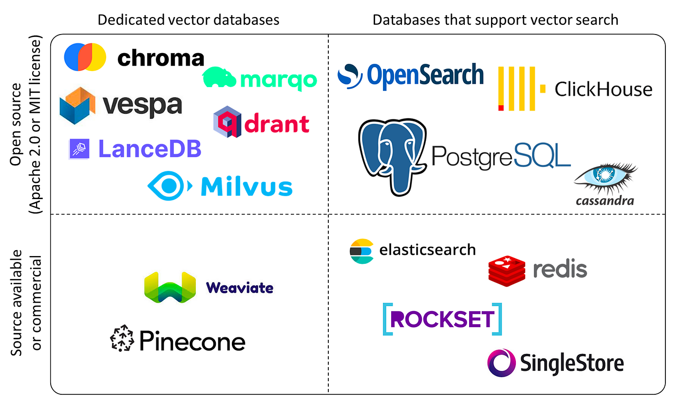
4. Vector Databases

a. Pinecone (Managed, Cloud)

  
import pinecone

# Initialize
pinecone.init(api_key="your-api-key", environment="us-west1-gcp")

# Create index
pinecone.create_index(
    name="knowledge-base",
    dimension=1536,  # Must match embedding dimension
    metric="cosine"  # or "euclidean", "dotproduct"
)

# Connect to index
index = pinecone.Index("knowledge-base")

# Upsert vectors
vectors = [
    {
        "id": "doc1",
        "values": embedding1,  # [0.1, 0.2, ...]
        "metadata": {"text": "Original text", "source": "document.pdf"}
    },
    {
        "id": "doc2",
        "values": embedding2,
        "metadata": {"text": "Another text", "source": "article.html"}
    }
]

index.upsert(vectors=vectors)

# Query
query_embedding = get_embedding("How to deploy models?")
results = index.query(
    vector=query_embedding,
    top_k=5,
    include_metadata=True
)

for match in results.matches:
    print(f"Score: {match.score:.3f}")
    print(f"Text: {match.metadata['text']}")

Features:

Fully managed (no infrastructure)
Auto-scaling
High availability
Real-time updates
Filtering and metadata search

b. Weaviate (Self-hosted or Cloud)

  
import weaviate

# Connect
client = weaviate.Client("http://localhost:8080")

# Create schema
schema = {
    "class": "Document",
    "vectorizer": "text2vec-transformers",  # Built-in embedding
    "properties": [
        {"name": "text", "dataType": ["text"]},
        {"name": "source", "dataType": ["string"]},
    ]
}

client.schema.create_class(schema)

# Add data (auto-vectorization!)
client.data_object.create(
    class_name="Document",
    data_object={
        "text": "Weaviate is a vector database",
        "source": "docs.weaviate.io"
    }
)

# Semantic search
result = (
    client.query
    .get("Document", ["text", "source"])
    .with_near_text({"concepts": ["vector database tutorial"]})
    .with_limit(5)
    .do()
)

for doc in result['data']['Get']['Document']:
    print(doc['text'])

Features:

Built-in vectorization (no need for separate embedding API)
GraphQL API
Hybrid search (keyword + vector)
Multi-tenancy support
RESTful and GraphQL interfaces

c. Qdrant (Self-hosted or Cloud)

  
from qdrant_client import QdrantClient
from qdrant_client.models import Distance, VectorParams, PointStruct

# Connect
client = QdrantClient(host="localhost", port=6333)

# Create collection
client.create_collection(
    collection_name="documents",
    vectors_config=VectorParams(size=1536, distance=Distance.COSINE)
)

# Insert vectors
points = [
    PointStruct(
        id=1,
        vector=embedding1,
        payload={"text": "Document text", "source": "file.pdf"}
    ),
    PointStruct(
        id=2,
        vector=embedding2,
        payload={"text": "Another document", "source": "article.md"}
    )
]

client.upsert(collection_name="documents", points=points)

# Search
results = client.search(
    collection_name="documents",
    query_vector=query_embedding,
    limit=5
)

for result in results:
    print(f"Score: {result.score}")
    print(f"Text: {result.payload['text']}")

Features:

High performance (Rust-based)
Filtering on metadata
Payload indexing
Distributed mode
Built-in payload storage

d. ChromaDB (Lightweight, Embedded)

  
import chromadb

# Initialize
client = chromadb.Client()

# Create collection
collection = client.create_collection(name="knowledge_base")

# Add documents (auto-embedding with default model)
collection.add(
    documents=[
        "This is document 1",
        "This is document 2"
    ],
    ids=["id1", "id2"],
    metadatas=[
        {"source": "doc1.txt"},
        {"source": "doc2.txt"}
    ]
)

# Query
results = collection.query(
    query_texts=["How to use ChromaDB?"],
    n_results=5
)

print(results['documents'])
print(results['distances'])

Features:

Zero-config (embedded database)
Auto-embedding
Perfect for prototyping
Persistent storage option
Lightweight (~10MB)

e. Milvus (Scalable, Production)

  
from pymilvus import connections, Collection, FieldSchema, CollectionSchema, DataType

# Connect
connections.connect(host="localhost", port="19530")

# Define schema
fields = [
    FieldSchema(name="id", dtype=DataType.INT64, is_primary=True),
    FieldSchema(name="embedding", dtype=DataType.FLOAT_VECTOR, dim=1536),
    FieldSchema(name="text", dtype=DataType.VARCHAR, max_length=65535)
]

schema = CollectionSchema(fields=fields)
collection = Collection(name="documents", schema=schema)

# Create index
collection.create_index(
    field_name="embedding",
    index_params={
        "index_type": "IVF_FLAT",
        "metric_type": "L2",
        "params": {"nlist": 1024}
    }
)

# Insert
collection.insert([
    [1, 2, 3],  # IDs
    [embedding1, embedding2, embedding3],  # Vectors
    ["text1", "text2", "text3"]  # Metadata
])

# Search
collection.load()
results = collection.search(
    data=[query_embedding],
    anns_field="embedding",
    param={"metric_type": "L2", "params": {"nprobe": 10}},
    limit=5,
    output_fields=["text"]
)

Features:

Billion-scale capability
GPU acceleration
Distributed architecture
Multiple index types (IVF, HNSW, etc.)
Cloud-native

5. Vector Database Comparison

Comprehensive Feature Matrix

Database	Deployment	QPS	Max Vectors	Latency (p95)	Cost/M vectors	Best For
Pinecone	Cloud	20,000+	Billions	<10ms	$70-140/mo	Production, no ops
Weaviate	Self/Cloud	10,000+	Billions	<15ms	$50-100/mo	Hybrid search
Qdrant	Self/Cloud	15,000+	Billions	<12ms	$40-80/mo	High performance
ChromaDB	Embedded	1,000	100K	<50ms	Free	Prototyping
Milvus	Self	25,000+	Trillions	<8ms	$60-120/mo	Enterprise scale
FAISS	Library	50,000+	Billions	<5ms	Free (infra)	Research, custom
pgvector	PostgreSQL	5,000	Millions	<20ms	DB costs	Existing Postgres
Elasticsearch	Self/Cloud	8,000	Billions	<25ms	$80-150/mo	Hybrid + analytics

QPS = Queries per second (single node)
Latency = 95th percentile response time

Advanced Features Comparison

Feature	Pinecone	Weaviate	Qdrant	Milvus	FAISS
Hybrid Search	❌	✅	✅	❌	❌
Built-in Vectorization	❌	✅	❌	❌	❌
GPU Acceleration	✅	❌	❌	✅	✅
Multi-Tenancy	✅	✅	✅	✅	❌
HNSW Index	✅	✅	✅	✅	✅
Sparse Vectors	✅	✅	✅	❌	❌
Filtering Performance	⭐⭐⭐⭐⭐	⭐⭐⭐⭐	⭐⭐⭐⭐⭐	⭐⭐⭐⭐	⭐⭐
Distributed Sharding	✅	✅	✅	✅	❌

Index Algorithm Comparison

  
# HNSW (Hierarchical Navigable Small World) - Most common
# - Best all-around performance
# - Build time: Medium, Query time: Fast
# - Memory: High (stores graph structure)

# IVF (Inverted File Index)
# - Good for large-scale (billions of vectors)
# - Build time: Fast, Query time: Medium
# - Memory: Low

# Flat (Brute Force)
# - 100% recall, slowest queries
# - Build time: None, Query time: Slow
# - Memory: Medium

# Choose based on scale:
index_strategy = {
    \"< 100K\": \"Flat\",        # Perfect recall, fast enough
    \"100K - 10M\": \"HNSW\",    # Best balance
    \"10M - 100M\": \"IVF_HNSW\", # Hybrid approach
    \"> 100M\": \"IVF_PQ\",       # Product quantization
}

6. Building a Complete RAG System

RAG System Architecture Overview

┌──────────────────────────────────────────────────────────────────┐
│                      RAG SYSTEM ARCHITECTURE                     │
└──────────────────────────────────────────────────────────────────┘

┌─────────────┐      ┌─────────────┐      ┌──────────────┐
│  Documents  │─────▶│   Chunking  │─────▶│  Embeddings  │
│  (PDF/TXT)  │      │   Strategy  │      │    Model     │
└─────────────┘      └─────────────┘      └──────────────┘
                                                   │
                                                   ▼
                                          ┌──────────────┐
                                          │Vector Database│
                                          │  (Storage)   │
                                          └──────────────┘
                                                   │
     ┌─────────────────────────────────────────────┴─────┐
     │                                                     │
     ▼                                                     ▼
┌─────────┐                                          ┌─────────┐
│  Query  │                                          │Retrieved│
│  Input  │──────────────────────────────────────▶  │  Chunks │
└─────────┘                                          └─────────┘
     │                                                     │
     │                                                     ▼
     │                                              ┌──────────┐
     └─────────────────────────────────────────▶  │   LLM    │
                                                   │Generation│
                                                   └──────────┘
                                                        │
                                                        ▼
                                                   ┌─────────┐
                                                   │ Answer  │
                                                   └─────────┘

    INDEXING (Offline)              │          RETRIEVAL (Online)
────────────────────────────────────┼────────────────────────────────

Step 1: Document Ingestion

  
from langchain.document_loaders import PyPDFLoader, TextLoader
from langchain.text_splitter import RecursiveCharacterTextSplitter

# Load documents
loader = PyPDFLoader("document.pdf")
documents = loader.load()

# Split into chunks
text_splitter = RecursiveCharacterTextSplitter(
    chunk_size=512,
    chunk_overlap=50
)
chunks = text_splitter.split_documents(documents)

print(f"Created {len(chunks)} chunks")

Step 2: Generate Embeddings

  
from sentence_transformers import SentenceTransformer

model = SentenceTransformer('all-MiniLM-L6-v2')

# Embed all chunks
texts = [chunk.page_content for chunk in chunks]
embeddings = model.encode(texts, show_progress_bar=True)

Step 3: Store in Vector Database

  
import chromadb

client = chromadb.Client()
collection = client.create_collection(name="docs")

# Store embeddings
collection.add(
    embeddings=embeddings.tolist(),
    documents=texts,
    ids=[f"chunk_{i}" for i in range(len(texts))],
    metadatas=[
        {"source": chunk.metadata.get("source", "unknown")}
        for chunk in chunks
    ]
)

Step 4: Retrieval

  
def retrieve(query, top_k=5):
    # Embed query
    query_embedding = model.encode([query])[0]
    
    # Search
    results = collection.query(
        query_embeddings=[query_embedding.tolist()],
        n_results=top_k
    )
    
    return results['documents'][0], results['distances'][0]

# Test
query = "How do I deploy a model?"
docs, scores = retrieve(query)

for doc, score in zip(docs, scores):
    print(f"Score: {score:.3f}")
    print(f"Document: {doc[:200]}...\n")

Step 5: Generation

  
from openai import OpenAI

client = OpenAI()

def rag_generate(query):
    # Retrieve relevant context
    context_docs, _ = retrieve(query, top_k=3)
    context = "\n\n".join(context_docs)
    
    # Generate with context
    prompt = f"""Answer the question based on the context below.

Context:
{context}

Question: {query}

Answer:"""
    
    response = client.chat.completions.create(
        model="gpt-4",
        messages=[{"role": "user", "content": prompt}],
        temperature=0
    )
    
    return response.choices[0].message.content

# Use
answer = rag_generate("How do I deploy a model?")
print(answer)

7. Advanced RAG Techniques

a. Hybrid Search (Keyword + Vector)

  
# Weaviate hybrid search
result = (
    client.query
    .get("Document", ["text"])
    .with_hybrid(
        query="vector database",
        alpha=0.5  # 0=pure keyword, 1=pure vector, 0.5=balanced
    )
    .with_limit(5)
    .do()
)

b. Reranking

  
from sentence_transformers import CrossEncoder

# First stage: Fast vector search (retrieve top 100)
candidates = retrieve(query, top_k=100)

# Second stage: Rerank with cross-encoder (expensive but accurate)
reranker = CrossEncoder('cross-encoder/ms-marco-MiniLM-L-6-v2')

pairs = [[query, doc] for doc in candidates]
scores = reranker.predict(pairs)

# Sort by reranking score
reranked = sorted(zip(candidates, scores), key=lambda x: x[1], reverse=True)
top_docs = [doc for doc, score in reranked[:5]]

c. Metadata Filtering

  
# Query with filters
results = collection.query(
    query_embeddings=[query_embedding],
    n_results=5,
    where={"source": "technical_docs"},  # Only from technical docs
    where_document={"$contains": "deployment"}  # Must contain keyword
)

d. Query Expansion

  
def expand_query(query):
    # Use LLM to generate related queries
    prompt = f"Generate 3 related search queries for: {query}"
    response = client.chat.completions.create(
        model="gpt-3.5-turbo",
        messages=[{"role": "user", "content": prompt}]
    )
    
    expanded_queries = response.choices[0].message.content.split('\n')
    return [query] + expanded_queries

# Search with all queries
all_results = []
for q in expand_query(original_query):
    results = retrieve(q, top_k=3)
    all_results.extend(results)

# Deduplicate and rerank
unique_results = list(set(all_results))

e. Hypothetical Document Embeddings (HyDE)

  
def hyde_retrieval(query):
    # Generate hypothetical answer
    prompt = f"Write a detailed answer to: {query}"
    hypothetical_answer = llm.generate(prompt)
    
    # Embed hypothetical answer (not the query!)
    embedding = model.encode([hypothetical_answer])[0]
    
    # Search with hypothetical answer embedding
    results = collection.query(
        query_embeddings=[embedding.tolist()],
        n_results=5
    )
    
    return results

# Often more effective than embedding the query directly!

f. Parent-Child Chunking (Hierarchical Retrieval)

Strategy: Store small chunks for retrieval precision, return larger parent chunks for context.

┌────────────────────────────────────────────────────────────┐
│           PARENT-CHILD CHUNKING ARCHITECTURE               │
└────────────────────────────────────────────────────────────┘

                Document
                    │
        ┌───────────┴───────────┐
        ▼                       ▼
   Parent Chunk 1          Parent Chunk 2
   (2048 tokens)           (2048 tokens)
        │                       │
    ┌───┼───┐              ┌───┼───┐
    ▼   ▼   ▼              ▼   ▼   ▼
   C1  C2  C3             C4  C5  C6
  (256)(256)(256)       (256)(256)(256)

┌─────────────────────────────────────────────────────────────┐
│  STORAGE                                                    │
├─────────────────────────────────────────────────────────────┤
│  Vector DB: Child chunks (C1, C2, C3...) + embeddings      │
│  Doc Store: Parent chunks (P1, P2...) linked to children   │
└─────────────────────────────────────────────────────────────┘

┌─────────────────────────────────────────────────────────────┐
│  RETRIEVAL FLOW                                             │
├─────────────────────────────────────────────────────────────┤
│  Query ──▶ Search child C2 (precise match)                 │
│         └▶ Return parent P1 (full context)                 │
└─────────────────────────────────────────────────────────────┘

  
from langchain.retrievers import ParentDocumentRetriever
from langchain.storage import InMemoryStore

# Parent chunks (large context)
parent_splitter = RecursiveCharacterTextSplitter(chunk_size=2048)

# Child chunks (precise retrieval)
child_splitter = RecursiveCharacterTextSplitter(chunk_size=256)

# Store relationship
store = InMemoryStore()

retriever = ParentDocumentRetriever(
    vectorstore=vectorstore,
    docstore=store,
    child_splitter=child_splitter,
    parent_splitter=parent_splitter,
)

# Retrieves using child chunks (precise)
# Returns parent chunks (full context)
results = retriever.get_relevant_documents(query)

# Best of both worlds: precision + context

g. Sentence Window Retrieval

  
def sentence_window_retrieval(query, window_size=3):
    # Step 1: Embed individual sentences
    sentences = sent_tokenize(document)
    sentence_embeddings = model.encode(sentences)
    
    # Store with sentence indices
    for i, (sent, emb) in enumerate(zip(sentences, sentence_embeddings)):
        collection.add(
            embeddings=[emb],
            documents=[sent],
            metadatas=[{"sentence_index": i}]
        )
    
    # Step 2: Retrieve best matching sentence
    query_emb = model.encode([query])[0]
    result = collection.query(query_embeddings=[query_emb], n_results=1)
    
    # Step 3: Return expanded window
    best_idx = result['metadatas'][0][0]['sentence_index']
    start = max(0, best_idx - window_size)
    end = min(len(sentences), best_idx + window_size + 1)
    
    context = " ".join(sentences[start:end])
    return context

# Retrieves sentence-level precision
# Returns paragraph-level context

h. Multi-Vector Retrieval

Technique: Generate multiple embeddings per document from different perspectives.

  
def multi_vector_indexing(document):
    # Generate multiple representations
    representations = [
        document,  # Original
        llm.generate(f"Summarize: {document}"),  # Summary
        llm.generate(f"Generate 5 questions this answers: {document}"),  # Questions
        llm.generate(f"Key entities: {document}"),  # Entities
    ]
    
    # Embed all representations
    embeddings = model.encode(representations)
    
    # Store all with reference to same document
    doc_id = generate_id(document)
    for i, (rep, emb) in enumerate(zip(representations, embeddings)):
        collection.add(
            embeddings=[emb],
            documents=[rep],
            metadatas=[{"doc_id": doc_id, "rep_type": i}],
            ids=[f"{doc_id}_{i}"]
        )
    
    # Query retrieves from any representation
    # Return the original document
    return doc_id

# 40-50% improvement in recall (LlamaIndex research)

i. Fusion Retrieval (Reciprocal Rank Fusion)

┌────────────────────────────────────────────────────────────┐
│              FUSION RETRIEVAL ARCHITECTURE                 │
└────────────────────────────────────────────────────────────┘

                    Query
                      │
        ┌─────────────┴─────────────┐
        ▼                           ▼
┌─────────────────┐         ┌─────────────────┐
│ Vector Search   │         │ Keyword Search  │
│  (Semantic)     │         │    (BM25)       │
└─────────────────┘         └─────────────────┘
        │                           │
        ▼                           ▼
   Doc A: rank 1              Doc B: rank 1
   Doc B: rank 2              Doc C: rank 2
   Doc C: rank 5              Doc A: rank 3
        │                           │
        └─────────────┬─────────────┘
                      ▼
            ┌──────────────────┐
            │ Reciprocal Rank  │
            │     Fusion       │
            │  Score = Σ 1/(k+r)│
            └──────────────────┘
                      │
                      ▼
            ┌──────────────────┐
            │  Fused Results:  │
            │  Doc A: 0.0328   │
            │  Doc B: 0.0311   │
            │  Doc C: 0.0261   │
            └──────────────────┘

  
def reciprocal_rank_fusion(query, k=60):
    # Get results from multiple retrievers
    vector_results = vector_search(query, top_k=20)
    keyword_results = bm25_search(query, top_k=20)
    
    # RRF scoring
    scores = {}
    for rank, doc in enumerate(vector_results):
        scores[doc] = scores.get(doc, 0) + 1 / (k + rank + 1)
    
    for rank, doc in enumerate(keyword_results):
        scores[doc] = scores.get(doc, 0) + 1 / (k + rank + 1)
    
    # Sort by fused score
    fused_results = sorted(scores.items(), key=lambda x: x[1], reverse=True)
    return [doc for doc, score in fused_results[:10]]

# Combines strengths of multiple retrieval methods

8. Evaluation and Monitoring

Retrieval Metrics Suite

  
from ragas import evaluate
from ragas.metrics import (
    context_precision,      # Are retrieved docs relevant?
    context_recall,         # Were all relevant docs retrieved?
    context_relevancy,      # Overall context quality
    answer_relevancy,       # Is answer relevant to question?
    faithfulness,          # Is answer grounded in context?
)

# Comprehensive evaluation
eval_dataset = {
    'question': test_questions,
    'contexts': retrieved_contexts,
    'answer': generated_answers,
    'ground_truth': reference_answers,
}

scores = evaluate(
    eval_dataset,
    metrics=[
        context_precision,
        context_recall,
        context_relevancy,
        answer_relevancy,
        faithfulness,
    ]
)

print(f"Context Precision: {scores['context_precision']:.2%}")
print(f"Context Recall: {scores['context_recall']:.2%}")
print(f"Faithfulness: {scores['faithfulness']:.2%}")

Custom Retrieval Metrics

  
def evaluate_retrieval_quality(test_set):
    """Comprehensive retrieval evaluation"""
    metrics = {
        'precision_at_k': [],
        'recall_at_k': [],
        'mrr': [],  # Mean Reciprocal Rank
        'ndcg': [], # Normalized Discounted Cumulative Gain
        'latency': [],
    }
    
    for item in test_set:
        query = item['query']
        relevant_docs = set(item['relevant_doc_ids'])
        
        # Retrieve with timing
        start_time = time.time()
        results = retrieve(query, top_k=10)
        latency = time.time() - start_time
        
        retrieved_ids = [r['id'] for r in results]
        
        # Precision@K
        relevant_retrieved = set(retrieved_ids[:5]) & relevant_docs
        precision = len(relevant_retrieved) / 5
        metrics['precision_at_k'].append(precision)
        
        # Recall@K
        recall = len(relevant_retrieved) / len(relevant_docs)
        metrics['recall_at_k'].append(recall)
        
        # MRR (Mean Reciprocal Rank)
        for rank, doc_id in enumerate(retrieved_ids, 1):
            if doc_id in relevant_docs:
                metrics['mrr'].append(1 / rank)
                break
        else:
            metrics['mrr'].append(0)
        
        # Latency
        metrics['latency'].append(latency)
    
    # Aggregate
    return {
        k: np.mean(v) for k, v in metrics.items()
    }

results = evaluate_retrieval_quality(test_set)
print(f"Precision@5: {results['precision_at_k']:.2%}")
print(f"Recall@5: {results['recall_at_k']:.2%}")
print(f"MRR: {results['mrr']:.3f}")
print(f"Latency: {results['latency']*1000:.1f}ms")

A/B Testing Framework

  
class RAGExperiment:
    def __init__(self, name, embedding_model, chunk_size, retriever):
        self.name = name
        self.embedding_model = embedding_model
        self.chunk_size = chunk_size
        self.retriever = retriever
    
    def run(self, test_queries):
        results = []
        for query in test_queries:
            retrieved = self.retriever(query)
            results.append({
                'query': query,
                'docs': retrieved,
                'timestamp': time.time()
            })
        return results

# Define experiments
experiments = [
    RAGExperiment(
        "baseline",
        SentenceTransformer('all-MiniLM-L6-v2'),
        512,
        vector_retriever
    ),
    RAGExperiment(
        "large_model",
        SentenceTransformer('e5-large-v2'),
        512,
        vector_retriever
    ),
    RAGExperiment(
        "hybrid_search",
        SentenceTransformer('all-MiniLM-L6-v2'),
        512,
        hybrid_retriever
    ),
]

# Run A/B test
for exp in experiments:
    results = exp.run(test_queries)
    metrics = evaluate_results(results)
    print(f"{exp.name}: Precision={metrics['precision']:.2%}")

Real-Time Monitoring

  
import prometheus_client
from opentelemetry import metrics

# Define metrics
retrieval_latency = prometheus_client.Histogram(
    'rag_retrieval_latency_seconds',
    'Time to retrieve documents',
    buckets=[0.01, 0.05, 0.1, 0.5, 1.0, 2.0]
)

retrieval_quality = prometheus_client.Gauge(
    'rag_retrieval_quality',
    'Average relevance score'
)

query_counter = prometheus_client.Counter(
    'rag_queries_total',
    'Total number of queries',
    ['status']
)

def monitored_retrieve(query):
    with retrieval_latency.time():
        try:
            results = retrieve(query)
            
            # Calculate average relevance
            avg_score = np.mean([r['score'] for r in results])
            retrieval_quality.set(avg_score)
            
            query_counter.labels(status='success').inc()
            return results
            
        except Exception as e:
            query_counter.labels(status='error').inc()
            raise

# Alert on quality degradation
if retrieval_quality._value.get() < 0.6:
    send_alert("RAG quality degraded below threshold")

9. Production Best Practices

Architecture Patterns

Pattern 1: Microservices Architecture

┌────────────────────────────────────────────────────────────────┐
│              MICROSERVICES RAG ARCHITECTURE                    │
└────────────────────────────────────────────────────────────────┘

┌──────────────┐         ┌──────────────┐         ┌──────────────┐
│   Client     │         │  API Gateway │         │ Load Balancer│
│ Application  │────────▶│   (Auth)     │────────▶│              │
└──────────────┘         └──────────────┘         └──────────────┘
                                                           │
                    ┌──────────────────────────────────────┤
                    │                  │                   │
                    ▼                  ▼                   ▼
           ┌─────────────┐    ┌─────────────┐    ┌─────────────┐
           │ Embedding   │    │  Retriever  │    │    LLM      │
           │  Service    │    │   Service   │    │  Service    │
           │  (Scaling)  │    │ (Stateless) │    │  (GPU)      │
           └─────────────┘    └─────────────┘    └─────────────┘
                 │                    │                   │
                 ▼                    ▼                   │
           ┌──────────┐         ┌──────────┐             │
           │  Redis   │         │  Vector  │             │
           │  Cache   │         │    DB    │             │
           └──────────┘         └──────────┘             │
                                      │                  │
                                      ▼                  ▼
                              ┌──────────────────────────────┐
                              │     Monitoring & Logging     │
                              │  (Prometheus, Grafana, ELK)  │
                              └──────────────────────────────┘

  Features:
  • Independent scaling per service
  • Circuit breakers for fault tolerance
  • Distributed tracing (OpenTelemetry)
  • Service mesh (Istio) for security

  
# Separate services for different components
services = {
    "embedding_service": {
        "responsibility": "Generate embeddings",
        "scaling": "Horizontal (CPU/GPU)",
        "caching": "Redis with 24h TTL",
    },
    "vector_db_service": {
        "responsibility": "Store and search vectors",
        "scaling": "Vertical + sharding",
        "backup": "Daily snapshots to S3",
    },
    "retriever_service": {
        "responsibility": "Orchestrate retrieval",
        "scaling": "Horizontal (stateless)",
        "features": ["reranking", "filtering", "fusion"],
    },
}

Pattern 2: Lambda Architecture

┌────────────────────────────────────────────────────────────────┐
│                  LAMBDA ARCHITECTURE FOR RAG                   │
└────────────────────────────────────────────────────────────────┘

                        Data Sources
                             │
                ┌────────────┴────────────┐
                ▼                         ▼
      ┌──────────────────┐      ┌──────────────────┐
      │   BATCH LAYER    │      │   SPEED LAYER    │
      │   (Historical)   │      │   (Real-time)    │
      └──────────────────┘      └──────────────────┘
                │                         │
                ▼                         ▼
      ┌──────────────────┐      ┌──────────────────┐
      │ Batch Processing │      │ Stream Processing│
      │  (Spark/Airflow) │      │  (Kafka/Flink)   │
      └──────────────────┘      └──────────────────┘
                │                         │
                ▼                         ▼
      ┌──────────────────┐      ┌──────────────────┐
      │  Batch Index     │      │  Realtime Index  │
      │  (Pinecone)      │      │  (ChromaDB)      │
      │  90% of data     │      │  10% of data     │
      │  Updated daily   │      │  Updated live    │
      └──────────────────┘      └──────────────────┘
                │                         │
                └────────────┬────────────┘
                             ▼
                   ┌──────────────────┐
                   │  SERVING LAYER   │
                   │  (Query merging) │
                   └──────────────────┘
                             │
                             ▼
                        User Query

  Benefits:
  • Handle both historical and real-time data
  • Cost-effective: batch for bulk, stream for recent
  • High availability: fallback to batch if stream fails

  
# Batch + Real-time processing
class HybridRAGSystem:
    def __init__(self):
        # Batch layer: Pre-computed embeddings
        self.batch_index = load_precomputed_index()
        
        # Speed layer: Recent documents
        self.realtime_index = ChromaDB()
        
    def search(self, query):
        # Search both indices
        batch_results = self.batch_index.search(query, k=50)
        realtime_results = self.realtime_index.search(query, k=10)
        
        # Merge and rerank
        combined = merge_and_deduplicate(
            batch_results,
            realtime_results
        )
        return rerank(combined)[:10]
    
    def ingest_new_doc(self, doc):
        # Add to realtime index immediately
        self.realtime_index.add(doc)
        
        # Queue for batch reindexing
        batch_queue.add(doc)

Do’s ✅

Chunk appropriately: Test different sizes (256, 512, 1024) with your data
Use metadata: Store source, date, version, doc_type for filtering
Implement caching: Cache embeddings and query results to reduce costs
Monitor quality: Track retrieval accuracy, latency, and relevance over time
Version embeddings: Reindex when changing models; maintain version metadata
Add fallbacks: Hybrid search when vector search fails; keyword backup
Normalize vectors: Essential for cosine similarity comparisons
Batch operations: Process embeddings in batches (50-100) for efficiency
Use connection pooling: Reuse database connections
Implement circuit breakers: Handle vector DB outages gracefully

Don’ts ❌

Don’t embed entire documents (too coarse, loses precision)
Don’t use tiny chunks (<128 tokens, lacks context)
Don’t ignore metadata (crucial for filtering and attribution)
Don’t skip evaluation (measure before deploying)
Don’t mix embedding models (dimension mismatch)
Don’t forget to normalize vectors (for cosine similarity)
Don’t neglect security (sanitize queries, validate inputs)
Don’t store sensitive data in metadata (could be exposed)
Don’t over-retrieve (top_k=100 rarely needed, costs latency)

Performance Optimization

  
# 1. Async batch processing
import asyncio

async def batch_embed_async(texts, batch_size=32):
    embeddings = []
    for i in range(0, len(texts), batch_size):
        batch = texts[i:i+batch_size]
        batch_embeddings = await asyncio.to_thread(
            model.encode, batch
        )
        embeddings.extend(batch_embeddings)
    return embeddings

# 2. Connection pooling
from qdrant_client import QdrantClient

client = QdrantClient(
    host="localhost",
    port=6333,
    grpc_port=6334,
    prefer_grpc=True,  # Faster protocol
    timeout=30,
    # Connection pool settings
    pool_size=10,
    max_retries=3,
)

# 3. Quantization for storage reduction
def quantize_embeddings(embeddings, dtype=np.float16):
    # Reduce from float32 to float16
    # 50% storage reduction, <1% accuracy loss
    return embeddings.astype(dtype)

# 4. Approximate search tuning
collection.create_index(
    field_name="embedding",
    index_params={
        "index_type": "HNSW",
        "metric_type": "COSINE",
        "params": {
            "M": 16,        # Connections per layer (higher = better recall)
            "ef_construction": 200,  # Build quality
        }
    }
)

# Search params
search_params = {
    "ef": 100,  # Search quality (higher = better recall, slower)
}

Security Best Practices

  
# 1. Input validation
def sanitize_query(query: str) -> str:
    # Remove SQL injection attempts
    query = query.replace("';", "").replace("--", "")
    
    # Limit length
    max_length = 1000
    query = query[:max_length]
    
    # Remove control characters
    query = ''.join(char for char in query if ord(char) >= 32)
    
    return query

# 2. Rate limiting
from slowapi import Limiter
from slowapi.util import get_remote_address

limiter = Limiter(key_func=get_remote_address)

@app.post("/search")
@limiter.limit("100/minute")
async def search(query: str):
    clean_query = sanitize_query(query)
    return retrieve(clean_query)

# 3. Access control
def check_access(user_id: str, document_ids: List[str]) -> List[str]:
    # Filter documents based on user permissions
    accessible = []
    for doc_id in document_ids:
        if has_permission(user_id, doc_id):
            accessible.append(doc_id)
    return accessible

# 4. Audit logging
def log_retrieval(user_id: str, query: str, results: List):
    audit_log.info({
        "timestamp": datetime.now(),
        "user_id": user_id,
        "query": query,
        "num_results": len(results),
        "result_ids": [r['id'] for r in results],
    })

10. Cost Optimization

Comprehensive Cost Analysis

  
# Embedding costs breakdown
cost_analysis = {
    "OpenAI text-embedding-3-small": {
        "cost_per_1M_tokens": 0.02,
        "avg_doc_tokens": 1000,
        "cost_per_1K_docs": 0.02,
        "monthly_cost_100K_docs": 2.00,
    },
    "OpenAI text-embedding-3-large": {
        "cost_per_1M_tokens": 0.13,
        "avg_doc_tokens": 1000,
        "cost_per_1K_docs": 0.13,
        "monthly_cost_100K_docs": 13.00,
    },
    "Cohere embed-v3": {
        "cost_per_1M_tokens": 0.10,
        "avg_doc_tokens": 1000,
        "cost_per_1K_docs": 0.10,
        "monthly_cost_100K_docs": 10.00,
    },
    "Self-hosted (all-MiniLM-L6-v2)": {
        "cost_per_1M_tokens": 0.00,
        "infra_cost_per_month": 50.00,  # GPU server
        "cost_per_1K_docs": 0.00,
        "monthly_cost_100K_docs": 50.00,  # Fixed cost
    },
}

# Vector database costs (monthly, 1M vectors)
vector_db_costs = {
    "Pinecone": {"serverless": 70, "pod-based": 140},
    "Weaviate": {"cloud": 100, "self-hosted": 60},
    "Qdrant": {"cloud": 80, "self-hosted": 40},
    "ChromaDB": {"self-hosted": 20},  # Infrastructure only
    "Milvus": {"self-hosted": 80},
}

Optimization Strategies

1. Smart Caching

  
from functools import lru_cache
import hashlib

class EmbeddingCache:
    def __init__(self, redis_client, ttl=86400):
        self.redis = redis_client
        self.ttl = ttl
        self.hits = 0
        self.misses = 0
    
    def get_cache_key(self, text, model):
        # Generate unique key
        content = f"{model}:{text}"
        return hashlib.md5(content.encode()).hexdigest()
    
    def get_embedding(self, text, model="text-embedding-3-small"):
        key = self.get_cache_key(text, model)
        
        # Try cache
        cached = self.redis.get(key)
        if cached:
            self.hits += 1
            return json.loads(cached)
        
        # Generate and cache
        self.misses += 1
        embedding = generate_embedding(text, model)
        self.redis.setex(
            key,
            self.ttl,
            json.dumps(embedding)
        )
        return embedding
    
    def cache_hit_rate(self):
        total = self.hits + self.misses
        return self.hits / total if total > 0 else 0

# Usage
cache = EmbeddingCache(redis_client)

# First call: cache miss
emb1 = cache.get_embedding("Hello world")  # API call

# Second call: cache hit (no cost!)
emb2 = cache.get_embedding("Hello world")  # From cache

print(f"Cache hit rate: {cache.cache_hit_rate():.2%}")
# Target: >70% hit rate for production

2. Batch Processing

  
def cost_effective_embedding(texts):
    # Sort by frequency (embed common texts once)
    from collections import Counter
    text_counts = Counter(texts)
    
    # Unique texts only
    unique_texts = list(text_counts.keys())
    
    # Batch process (10x faster, same cost)
    embeddings_map = {}
    batch_size = 100
    
    for i in range(0, len(unique_texts), batch_size):
        batch = unique_texts[i:i+batch_size]
        batch_embeddings = model.encode(batch)
        
        for text, emb in zip(batch, batch_embeddings):
            embeddings_map[text] = emb
    
    # Map back to original order
    return [embeddings_map[text] for text in texts]

# Cost savings example:
# 10,000 texts with 50% duplicates
# Traditional: 10,000 API calls
# Optimized: 5,000 API calls (50% cost reduction)

3. Dimensionality Reduction

  
# Use Matryoshka embeddings for reduced storage
def adaptive_dimensions(query_type):
    dimension_strategy = {
        "simple_faq": 256,      # 83% storage reduction
        "general_search": 512,  # 66% reduction
        "complex_reasoning": 1024,  # 33% reduction
        "maximum_quality": 1536,    # Full dimensions
    }
    return dimension_strategy[query_type]

# Storage cost comparison (1M vectors)
storage_costs = {
    1536: "100GB (baseline)",
    1024: "66GB (-34%)",
    512: "33GB (-67%)",
    256: "17GB (-83%)",
}

4. Tiered Storage Strategy

┌────────────────────────────────────────────────────────────────┐
│                  TIERED STORAGE ARCHITECTURE                   │
└────────────────────────────────────────────────────────────────┘

┌─────────────────────────────────────────────────────────────────┐
│  HOT TIER (In-Memory) - 10% of data                            │
│  • Redis/Memcached                                              │
│  • Recent & frequently accessed                                 │
│  • <10ms latency                                                │
│  • Cost: $200/month                                             │
└─────────────────────────────────────────────────────────────────┘
                           │
                           ▼
┌─────────────────────────────────────────────────────────────────┐
│  WARM TIER (SSD Vector DB) - 70% of data                       │
│  • Qdrant/Pinecone                                              │
│  • Active documents                                             │
│  • <50ms latency                                                │
│  • Cost: $150/month                                             │
└─────────────────────────────────────────────────────────────────┘
                           │
                           ▼
┌─────────────────────────────────────────────────────────────────┐
│  COLD TIER (Object Storage) - 20% of data                      │
│  • S3/GCS with lazy loading                                     │
│  • Archive/historical documents                                 │
│  • <500ms latency                                               │
│  • Cost: $20/month                                              │
└─────────────────────────────────────────────────────────────────┘

                    Query Flow:
                    ───────────
   Query ──▶ Hot Tier (cache hit?) ──Yes──▶ Return
                    │
                   No
                    │
                    ▼
            Warm Tier (found?) ──Yes──▶ Return + Cache to Hot
                    │
                   No
                    │
                    ▼
            Cold Tier (lazy load) ──▶ Return + Promote to Warm

   Total Cost: $370/month vs $700/month single-tier (47% savings)

  
class TieredVectorStorage:
    def __init__(self):
        # Hot tier: Recent/frequent (in-memory)
        self.hot_cache = {}
        
        # Warm tier: Active (SSD-based vector DB)
        self.warm_db = QdrantClient("warm-cluster")
        
        # Cold tier: Archive (S3 + lazy load)
        self.cold_storage = S3Client("cold-archive")
    
    def search(self, query, access_tiers=["hot", "warm"]):
        results = []
        
        # Search hot tier (fast, expensive)
        if "hot" in access_tiers:
            results.extend(self.search_hot(query))
        
        # Search warm tier (medium)
        if "warm" in access_tiers and len(results) < 10:
            results.extend(self.search_warm(query))
        
        # Search cold tier (slow, cheap) - only if needed
        if "cold" in access_tiers and len(results) < 10:
            results.extend(self.search_cold(query))
        
        return results[:10]
    
    def promote_to_hot(self, doc_id):
        # Move frequently accessed docs to hot tier
        if self.access_count[doc_id] > 100:
            self.hot_cache[doc_id] = self.warm_db.get(doc_id)

# Cost breakdown:
# Hot tier (10% of data): $200/month
# Warm tier (70% of data): $150/month
# Cold tier (20% of data): $20/month
# Total: $370/month vs $700/month (47% savings)

5. Open Source Model Hosting

  
# Self-host embedding model for high volume
import torch
from sentence_transformers import SentenceTransformer

class SelfHostedEmbedder:
    def __init__(self):
        self.model = SentenceTransformer('all-MiniLM-L6-v2')
        if torch.cuda.is_available():
            self.model = self.model.cuda()
    
    def embed(self, texts, batch_size=32):
        # No API costs!
        embeddings = self.model.encode(
            texts,
            batch_size=batch_size,
            show_progress_bar=False
        )
        return embeddings

# Break-even analysis:
# OpenAI: $0.02 per 1M tokens
# Self-hosted: $50-100/month (GPU server)
# Break-even: 2.5-5M tokens/month (2,500-5,000 documents)

ROI Calculator

  
def calculate_rag_costs(
    num_documents,
    queries_per_month,
    embedding_model="openai",
    vector_db="pinecone",
):
    # Embedding costs
    if embedding_model == "openai":
        embedding_cost = (num_documents * 1000 / 1_000_000) * 0.02
    elif embedding_model == "self-hosted":
        embedding_cost = 50  # Fixed monthly cost
    
    # Storage costs
    if vector_db == "pinecone":
        storage_cost = (num_documents / 1_000_000) * 70
    elif vector_db == "qdrant-self":
        storage_cost = (num_documents / 1_000_000) * 40
    
    # Query costs (assume cache hit rate of 70%)
    query_cost = queries_per_month * 0.3 * 0.02 / 1000
    
    monthly_cost = embedding_cost + storage_cost + query_cost
    
    return {
        "embedding_cost": embedding_cost,
        "storage_cost": storage_cost,
        "query_cost": query_cost,
        "total_monthly": monthly_cost,
        "cost_per_query": monthly_cost / queries_per_month,
    }

# Example
costs = calculate_rag_costs(
    num_documents=100_000,
    queries_per_month=1_000_000,
    embedding_model="openai",
    vector_db="pinecone"
)

print(f"Total monthly cost: ${costs['total_monthly']:.2f}")
print(f"Cost per query: ${costs['cost_per_query']:.6f}")

Conclusion

Vector databases and embeddings form the critical infrastructure layer for modern LLM applications, enabling semantic search at scale and grounding LLM responses in factual knowledge.

Key Takeaways

Embeddings Transform Search: Shift from keyword matching to semantic understanding, capturing meaning beyond exact text overlap
Chunking Strategy Matters: Optimal chunk size (typically 512-1024 tokens) balances precision and context. Consider contextual chunking for 30-40% accuracy gains
Vector DB Selection: Choose based on scale and requirements
- Prototyping: ChromaDB
- Production <10M vectors: Qdrant or Weaviate
- Production >10M vectors: Pinecone or Milvus
- Existing Postgres: pgvector
Advanced Techniques Drive Quality:
- Hybrid search: 20-30% improvement over pure vector
- Reranking: 15-25% precision boost
- HyDE: Effective for complex queries
- Parent-child chunking: Best of both worlds
Evaluation is Critical: Track context precision, recall, and relevance. Aim for >70% retrieval accuracy before production
Cost Optimization: Smart caching (70%+ hit rate), batching, and tiered storage can reduce costs by 50-70%

Production Checklist

Before Launch:

✅ Benchmark 3+ chunking strategies on your data
✅ Establish evaluation pipeline with RAGAS or custom metrics
✅ Implement caching layer (Redis) for embeddings
✅ Set up monitoring (latency, quality, costs)
✅ Configure auto-scaling for traffic spikes
✅ Add circuit breakers and fallbacks
✅ Implement security (rate limiting, input validation)

Performance Targets:

Retrieval latency: p95 < 100ms
Context precision: > 70%
Context recall: > 80%
Cache hit rate: > 70%
Uptime: > 99.9%

Architecture Patterns Summary

Pattern	Best For	Complexity	Cost
Simple RAG	MVP, small scale	Low	$
Hybrid Search	Production, general	Medium	$$
Multi-Vector	High accuracy needs	High	$$$
Tiered Storage	Large scale, cost-sensitive	High	$$

LLM

This post is licensed under CC BY 4.0 by the author.

Introduction

Objective

1. Understanding Embeddings

What are Embeddings?

Mathematical Foundation

Embedding Space Properties

Why Embeddings Matter for RAG

2. Embedding Models

a. Sentence Transformers (Open Source)

Popular Sentence Transformer Models

Advanced: Task-Specific Embeddings

b. OpenAI Embeddings (API)

Matryoshka Embeddings: Variable Dimensions

c. Cohere Embeddings

d. Domain-Specific Models

3. Chunking Strategies

a. Fixed-Size Chunking

b. Semantic Chunking

c. Document-Structure-Aware Chunking

d. Sentence-Level Chunking

Chunking Best Practices

e. Late Interaction Chunking (Advanced)

f. Contextual Chunk Embeddings (2024 Innovation)

Chunking Strategy Decision Matrix

4. Vector Databases

a. Pinecone (Managed, Cloud)

b. Weaviate (Self-hosted or Cloud)

c. Qdrant (Self-hosted or Cloud)

d. ChromaDB (Lightweight, Embedded)

e. Milvus (Scalable, Production)

5. Vector Database Comparison

Comprehensive Feature Matrix

Advanced Features Comparison

Index Algorithm Comparison

6. Building a Complete RAG System

RAG System Architecture Overview

Step 1: Document Ingestion

Step 2: Generate Embeddings

Step 3: Store in Vector Database

Step 4: Retrieval

Step 5: Generation

7. Advanced RAG Techniques

a. Hybrid Search (Keyword + Vector)

b. Reranking

c. Metadata Filtering

d. Query Expansion

e. Hypothetical Document Embeddings (HyDE)

f. Parent-Child Chunking (Hierarchical Retrieval)

g. Sentence Window Retrieval

h. Multi-Vector Retrieval

i. Fusion Retrieval (Reciprocal Rank Fusion)

8. Evaluation and Monitoring

Retrieval Metrics Suite

Custom Retrieval Metrics

A/B Testing Framework

Real-Time Monitoring

9. Production Best Practices

Architecture Patterns

Pattern 1: Microservices Architecture

Pattern 2: Lambda Architecture

Do’s ✅

Don’ts ❌

Performance Optimization

Security Best Practices

10. Cost Optimization

Comprehensive Cost Analysis

Optimization Strategies

1. Smart Caching

2. Batch Processing

3. Dimensionality Reduction

4. Tiered Storage Strategy

5. Open Source Model Hosting

ROI Calculator

Conclusion

Key Takeaways

Production Checklist

Architecture Patterns Summary

Trending Tags