Complete Guide to Reinforcement Learning: From Theory to Practice

Introduction

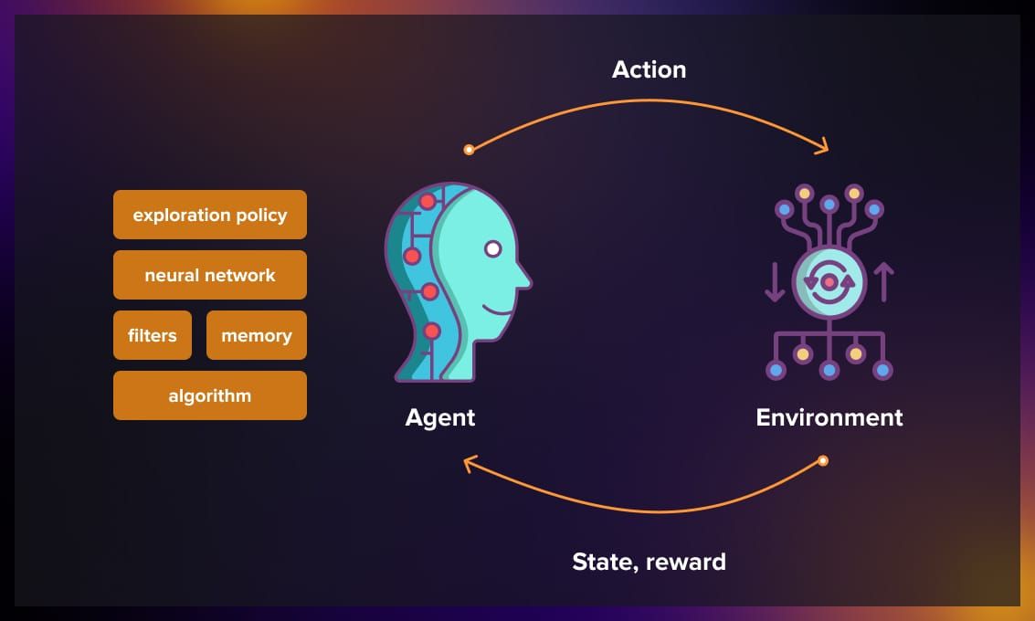
Reinforcement Learning (RL) is a branch of machine learning where an agent learns to make optimal decisions by interacting with its environment. Unlike supervised learning, the agent doesn’t have labeled examples but learns through rewards and punishments it receives.

Key Concepts

Agent: The entity that makes decisions

Environment: The world in which the agent operates

State: The current situation of the environment

Action: What the agent can do in a given state

Reward: The feedback received after an action

Policy: The agent’s strategy for choosing actions

Concrete Example: Robot Navigation

# Simple example: a robot navigating a grid
import numpy as np
import matplotlib.pyplot as plt

class SimpleGridWorld:
    def __init__(self, size=5):
        self.size = size
        self.state = [0, 0]  # Initial position
        self.goal = [4, 4]   # Goal position
        self.obstacles = [[2, 2], [2, 3], [3, 2]]  # Obstacles
        
    def reset(self):
        self.state = [0, 0]
        return self.state.copy()
    
    def step(self, action):
        # Actions: 0=up, 1=right, 2=down, 3=left
        old_state = self.state.copy()
        
        if action == 0 and self.state[0] > 0:  # Up
            self.state[0] -= 1
        elif action == 1 and self.state[1] < self.size-1:  # Right
            self.state[1] += 1
        elif action == 2 and self.state[0] < self.size-1:  # Down
            self.state[0] += 1
        elif action == 3 and self.state[1] > 0:  # Left
            self.state[1] -= 1
        
        # Check collisions with obstacles
        if self.state in self.obstacles:
            self.state = old_state
            reward = -10
        elif self.state == self.goal:
            reward = 100
        else:
            reward = -1  # Movement cost
        
        done = (self.state == self.goal)
        return self.state.copy(), reward, done
    
    def render(self):
        grid = np.zeros((self.size, self.size))
        grid[self.state[0], self.state[1]] = 1  # Agent
        grid[self.goal[0], self.goal[1]] = 2    # Goal
        for obs in self.obstacles:
            grid[obs[0], obs[1]] = -1  # Obstacles
        
        plt.imshow(grid, cmap='RdYlBu')
        plt.title(f'Position: {self.state}')
        plt.show()

# Test the environment
env = SimpleGridWorld()
state = env.reset()
print(f"Initial state: {state}")

# Simulate a few random steps
for i in range(5):
    action = np.random.randint(0, 4)
    state, reward, done = env.step(action)
    print(f"Action: {action}, New state: {state}, Reward: {reward}")
    if done:
        print("Goal reached!")
        break

2. Mathematical Foundations

2.1 Markov Decision Processes (MDP)

Markov Decision Processes (MDP) form the fundamental mathematical framework of Reinforcement Learning. They model situations where decisions influence future outcomes probabilistically.

Components of an MDP:

• S (States): All possible states in which the agent can be
  • Example: positions on a game board, robot configurations
• A (Actions): All actions the agent can perform
  • Example: up/down/left/right, accelerate/brake
• P (Transition function): Probability of moving from one state to another by performing an action
  • Models real-world uncertainty
  • Example: a robot going right might slightly deviate
• R (Reward function): Numerical feedback received after a transition
  • Guides agent learning
  • Example: +100 for reaching goal, -1 per movement
• γ (Discount factor): Value between 0 and 1 that determines the importance of future rewards
  • γ close to 0: agent is myopic (favors immediate rewards)
  • γ close to 1: agent is forward-looking (thinks long-term)

Markov Property: The optimal decision depends only on the current state, not the complete history.

Concrete example: In chess, to choose the best move, you only need the current position of pieces on the board. It doesn’t matter how you got to this position (after 10 moves or 50 moves), the best decision is the same. The current state contains all necessary information.

Bellman Equation

The Bellman equation is the fundamental equation of RL that expresses a simple recursive relationship:

“The value of being in a state = the immediate reward you can get + the (discounted) value of the state you arrive at next”

In other words, the value of a state is the sum of:

1. What you gain immediately
2. The future value (weighted by γ) you can obtain

This equation allows value information to propagate through all states, enabling the agent to understand which states are truly beneficial in the long term.

import numpy as np
from collections import defaultdict

class MDP:
    def __init__(self, states, actions, transitions, rewards, gamma=0.9):
        """
        Complete MDP with defined transitions and rewards
        
        Args:
            states: List of states
            actions: List of actions
            transitions: Dict {(state, action): {next_state: probability}}
            rewards: Dict {(state, action, next_state): reward}
            gamma: Discount factor
        """
        self.states = states
        self.actions = actions
        self.transitions = transitions
        self.rewards = rewards
        self.gamma = gamma
        
    def get_transitions(self, state, action):
        """Return possible transitions from (state, action)"""
        return self.transitions.get((state, action), {})
    
    def get_reward(self, state, action, next_state):
        """Return reward for a transition"""
        return self.rewards.get((state, action, next_state), 0)

# Example: Simple MDP with 3 states
states = ['S0', 'S1', 'S2']
actions = ['left', 'right']

# Define transitions: P(s'|s,a)
transitions = {
    ('S0', 'left'): {'S0': 0.8, 'S1': 0.2},
    ('S0', 'right'): {'S0': 0.1, 'S1': 0.9},
    ('S1', 'left'): {'S0': 0.5, 'S1': 0.5},
    ('S1', 'right'): {'S1': 0.3, 'S2': 0.7},
    ('S2', 'left'): {'S1': 0.4, 'S2': 0.6},
    ('S2', 'right'): {'S2': 1.0}
}

# Define rewards
rewards = {
    ('S0', 'left', 'S0'): -1,   ('S0', 'left', 'S1'): -1,
    ('S0', 'right', 'S0'): -1,  ('S0', 'right', 'S1'): -1,
    ('S1', 'left', 'S0'): -1,   ('S1', 'left', 'S1'): -1,
    ('S1', 'right', 'S1'): -1,  ('S1', 'right', 'S2'): 10,  # High reward!
    ('S2', 'left', 'S1'): -1,   ('S2', 'left', 'S2'): 0,
    ('S2', 'right', 'S2'): 0
}

mdp = MDP(states, actions, transitions, rewards)
print("MDP created successfully!")
print(f"States: {mdp.states}")
print(f"Actions: {mdp.actions}")

2.2 Dynamic Programming Algorithms

Dynamic Programming includes algorithms that compute the optimal policy when you perfectly know the environment model (transitions and rewards). These are planning methods rather than pure learning.

Value Iteration

Value Iteration directly computes the optimal value function by iteratively updating it for all states.

How it works:

1. Initialization: Start with arbitrary values for all states (often 0)

2. Iterative update: For each state, compute the best possible value considering all available actions. For each action, look at:
   • The expected immediate reward
   • The states this action can lead to (with their probabilities)
   • The value of these future states

3. Choose maximum: Keep the best value among all possible actions

4. Convergence: Repeat until values hardly change anymore (convergence)

5. Policy extraction: Once optimal values are found, the optimal policy simply consists of choosing, in each state, the action that leads to the best value

Advantages:

• Guaranteed to find the optimal policy
• Converges relatively quickly
• Simple to implement

Limitations:

• Requires knowing the complete model (transitions and rewards)
• Not practical for very large state spaces

def value_iteration(mdp, theta=0.001):
    """
    Value iteration algorithm
    
    Args:
        mdp: Markov Decision Process
        theta: Convergence threshold
    
    Returns:
        V: Optimal value function
        policy: Optimal policy
    """
    V = {state: 0 for state in mdp.states}
    
    iteration = 0
    while True:
        iteration += 1
        delta = 0
        old_V = V.copy()
        
        # Update each state
        for state in mdp.states:
            # Calculate maximum value over all actions
            action_values = []
            
            for action in mdp.actions:
                value = 0
                transitions = mdp.get_transitions(state, action)
                
                for next_state, prob in transitions.items():
                    reward = mdp.get_reward(state, action, next_state)
                    value += prob * (reward + mdp.gamma * old_V[next_state])
                
                action_values.append(value)
            
            if action_values:  # If actions are available
                V[state] = max(action_values)
                delta = max(delta, abs(V[state] - old_V[state]))
        
        print(f"Iteration {iteration}: δ = {delta:.6f}")
        if delta < theta:
            break
    
    # Extract optimal policy
    policy = {}
    for state in mdp.states:
        action_values = []
        
        for action in mdp.actions:
            value = 0
            transitions = mdp.get_transitions(state, action)
            
            for next_state, prob in transitions.items():
                reward = mdp.get_reward(state, action, next_state)
                value += prob * (reward + mdp.gamma * V[next_state])
            
            action_values.append((action, value))
        
        # Choose action with maximum value
        if action_values:
            policy[state] = max(action_values, key=lambda x: x[1])[0]
    
    return V, policy

# Apply Value Iteration
optimal_V, optimal_policy = value_iteration(mdp)

print("\n=== VALUE ITERATION RESULTS ===")
print("Optimal value function:")
for state in mdp.states:
    print(f"V*({state}) = {optimal_V[state]:.3f}")

print("\nOptimal policy:")
for state in mdp.states:
    print(f"π*({state}) = {optimal_policy[state]}")

Policy Iteration

Policy Iteration alternates between two phases: evaluating the current policy, then improving it. Rather than directly computing optimal values, it progressively improves a policy.

The two phases:

1. Policy Evaluation:
   • Calculates the value of each state by following the current policy
   • Answers the question: “If I follow this policy, what value can I expect?”
   • Uses the Bellman equation iteratively until convergence
2. Policy Improvement:
   • With the obtained values, creates a new policy
   • For each state, chooses the action that leads to the best value
   • If the new policy is identical to the old one, we’ve found the optimum!

Complete process:

Initial policy (random)
  ↓
Evaluate this policy → Values
  ↓
Improve policy with these values → New policy
  ↓
Policy changed? → Yes: Restart | No: Done!

Comparison Value Iteration vs Policy Iteration:

• Value Iteration: Updates values once per iteration (faster per iteration)
• Policy Iteration: Fully evaluates each policy before changing (fewer total iterations)

In practice: Policy Iteration often converges in fewer iterations than Value Iteration, but each iteration is more expensive.

def policy_evaluation(mdp, policy, theta=0.001):
    """Evaluate a given policy"""
    V = {state: 0 for state in mdp.states}
    
    while True:
        delta = 0
        old_V = V.copy()
        
        for state in mdp.states:
            if state in policy:
                action = policy[state]
                value = 0
                transitions = mdp.get_transitions(state, action)
                
                for next_state, prob in transitions.items():
                    reward = mdp.get_reward(state, action, next_state)
                    value += prob * (reward + mdp.gamma * old_V[next_state])
                
                V[state] = value
                delta = max(delta, abs(V[state] - old_V[state]))
        
        if delta < theta:
            break
    
    return V

def policy_improvement(mdp, V):
    """Policy improvement"""
    policy = {}
    
    for state in mdp.states:
        action_values = []
        
        for action in mdp.actions:
            value = 0
            transitions = mdp.get_transitions(state, action)
            
            for next_state, prob in transitions.items():
                reward = mdp.get_reward(state, action, next_state)
                value += prob * (reward + mdp.gamma * V[next_state])
            
            action_values.append((action, value))
        
        if action_values:
            policy[state] = max(action_values, key=lambda x: x[1])[0]
    
    return policy

def policy_iteration(mdp):
    """Policy iteration algorithm"""
    # Random initial policy
    policy = {state: mdp.actions[0] for state in mdp.states}
    
    iteration = 0
    while True:
        iteration += 1
        print(f"Policy iteration {iteration}")
        
        # Policy evaluation
        V = policy_evaluation(mdp, policy)
        
        # Policy improvement
        new_policy = policy_improvement(mdp, V)
        
        # Check convergence
        if policy == new_policy:
            print("Convergence reached!")
            break
        
        policy = new_policy
    
    return V, policy

# Apply Policy Iteration
pi_V, pi_policy = policy_iteration(mdp)

print("\n=== POLICY ITERATION RESULTS ===")
print("Value function:")
for state in mdp.states:
    print(f"V^π({state}) = {pi_V[state]:.3f}")

print("\nPolicy:")
for state in mdp.states:
    print(f"π({state}) = {pi_policy[state]}")

3. Classical Algorithms

3.1 Monte Carlo Methods

Monte Carlo methods are learning algorithms that estimate values by averaging complete returns obtained over multiple episodes. They take their name from the random simulations used in Monte Carlo casinos.

Fundamental principle: Instead of trying to predict what will happen at each step (like TD Learning), Monte Carlo waits for the complete end of an episode to see what actually happened. Then it averages all observed returns for each state or state-action pair encountered.

How it works:

1. Play complete episodes: The agent plays from start to finish, recording all states, actions and rewards
2. Calculate returns: At the end, calculate the total return (sum of discounted rewards) from each visited state
3. Average: Update value estimate by averaging all observed returns for each state

Two main variants:

• First-visit Monte Carlo: Counts each state only once per episode (the first visit)
• Every-visit Monte Carlo: Counts all visits to a state in an episode

Advantages:

• Conceptually simple: Uses real experience without a model
• Unbiased: Directly estimates true returns (no bootstrap approximation)
• Independent of transitions: No need to know transition probabilities
• Efficient for short episodes: Works well when episodes terminate quickly

Disadvantages:

• Requires complete episodes: Cannot learn online during an episode
• High variance: Returns can vary a lot between episodes
• Not suited for continuous tasks: Requires natural termination points

Recommended use cases:

• Games with short sessions (chess, go)
• Naturally episodic environments
• When unbiased estimates are wanted
• Systems where each episode gives a lot of information

import numpy as np
import random
from collections import defaultdict

class MonteCarloAgent:
    def __init__(self, env, epsilon=0.1, gamma=0.9):
        self.env = env
        self.epsilon = epsilon  # Exploration rate
        self.gamma = gamma      # Discount factor
        self.Q = defaultdict(lambda: defaultdict(float))  # Q-values
        self.returns = defaultdict(lambda: defaultdict(list))  # Returns for each (state, action)
        self.policy = defaultdict(int)  # Current policy
        
    def get_action(self, state, explore=True):
        """Epsilon-greedy policy"""
        if explore and random.random() < self.epsilon:
            return random.randint(0, 3)  # Random action
        else:
            # Greedy action: maximize Q(s,a)
            state_key = tuple(state)
            if state_key in self.Q:
                return max(self.Q[state_key], key=self.Q[state_key].get)
            return random.randint(0, 3)
    
    def generate_episode(self):
        """Generate a complete episode"""
        episode = []
        state = self.env.reset()
        
        while True:
            action = self.get_action(state)
            next_state, reward, done = self.env.step(action)
            
            episode.append((tuple(state), action, reward))
            state = next_state
            
            if done:
                break
        
        return episode
    
    def monte_carlo_control(self, num_episodes=1000):
        """Monte Carlo Control algorithm"""
        for episode_num in range(num_episodes):
            # Generate an episode
            episode = self.generate_episode()
            
            # Calculate returns
            G = 0  # Return
            visited = set()
            
            # Traverse episode in reverse
            for t in range(len(episode) - 1, -1, -1):
                state, action, reward = episode[t]
                G = self.gamma * G + reward
                
                # First-visit MC: consider only first visit
                if (state, action) not in visited:
                    visited.add((state, action))
                    
                    # Update returns
                    self.returns[state][action].append(G)
                    
                    # Update Q(s,a): average of returns
                    self.Q[state][action] = np.mean(self.returns[state][action])
                    
                    # Update policy (greedy)
                    if state in self.Q:
                        self.policy[state] = max(self.Q[state], key=self.Q[state].get)
            
            # Decrease epsilon (exploration decay)
            if episode_num % 100 == 0:
                self.epsilon = max(0.01, self.epsilon * 0.95)
                if episode_num % 500 == 0:
                    print(f"Episode {episode_num}, epsilon: {self.epsilon:.3f}")
        
        return self.Q, self.policy

# Test with our grid environment
env = SimpleGridWorld(size=5)
mc_agent = MonteCarloAgent(env)

print("Monte Carlo training...")
Q_values, policy = mc_agent.monte_carlo_control(num_episodes=2000)

print("\nQ-value examples:")
for state in list(Q_values.keys())[:5]:
    print(f"Q{state}: {dict(Q_values[state])}")

3.2 Temporal Difference Learning

Simple definition: Temporal Difference (TD) Learning is a learning method that updates its estimates at each time step based on the difference between its current prediction and what actually happened. It’s like continuously adjusting your compass during a journey rather than waiting to arrive at your destination.

Temporal Difference (TD) is an approach that combines ideas from Monte Carlo and dynamic programming. Unlike Monte Carlo which waits for the end of an episode, TD learns directly at each step by estimating the future value.

Principle: TD Learning uses the difference between two successive estimates (called “TD error”) to update its values. Instead of collecting all rewards until the end, it estimates what might happen next and adjusts its beliefs immediately.

Advantages over Monte Carlo:

• Online learning: No need to wait for the end of an episode
• Efficient for continuous tasks: Works even without termination point
• Faster convergence: Uses each transition immediately
• Lower variance: Bootstrap reduces noise in estimates

Disadvantage:

• Initial bias: Bootstrap estimates may be incorrect at the start
• Depends on estimate quality: If estimated values are bad, learning can be slow

3.2.1 Q-Learning

Simple definition: Q-Learning is the most famous RL algorithm. It learns a “quality table” (Q-table) that tells the agent what is the best action in each situation. The “Q” means “Quality” - it’s the quality of an action in a given state.

Q-Learning is an off-policy algorithm that learns the optimal action-value function Q*(s,a) independently of the policy followed.

How the update works: The agent adjusts its Q-value using the received reward plus the best estimated value of the next state, progressively correcting its estimate with a learning rate alpha. At each step, it updates its knowledge by combining the old estimate with new information obtained.

Main characteristics:

• Off-policy: Can learn the optimal policy while exploring with another policy
• Guaranteed convergence: Converges to Q* under certain conditions
• No model required: Learns directly from experience
• Epsilon-greedy exploration: Balance between exploitation and exploration

class QLearningAgent:
    def __init__(self, env, alpha=0.1, epsilon=0.1, gamma=0.9):
        self.env = env
        self.alpha = alpha      # Learning rate
        self.epsilon = epsilon  # Exploration rate
        self.gamma = gamma      # Discount factor
        self.Q = defaultdict(lambda: defaultdict(float))
        
    def get_action(self, state, explore=True):
        """Epsilon-greedy policy"""
        state_key = tuple(state)
        
        if explore and random.random() < self.epsilon:
            return random.randint(0, 3)  # Exploration
        else:
            # Exploitation: choose action with max Q
            if state_key in self.Q and self.Q[state_key]:
                return max(self.Q[state_key], key=self.Q[state_key].get)
            return random.randint(0, 3)
    
    def update_q_value(self, state, action, reward, next_state):
        """Q-learning update"""
        state_key = tuple(state)
        next_state_key = tuple(next_state)
        
        # Q(s,a) ← Q(s,a) + α[r + γ max_a' Q(s',a') - Q(s,a)]
        current_q = self.Q[state_key][action]
        
        # Find max Q(s', a') for next state
        if next_state_key in self.Q and self.Q[next_state_key]:
            max_next_q = max(self.Q[next_state_key].values())
        else:
            max_next_q = 0
        
        # Q-learning update
        target = reward + self.gamma * max_next_q
        self.Q[state_key][action] = current_q + self.alpha * (target - current_q)
    
    def train(self, num_episodes=1000):
        """Q-learning training"""
        rewards_per_episode = []
        
        for episode in range(num_episodes):
            state = self.env.reset()
            total_reward = 0
            steps = 0
            max_steps = 100  # Avoid infinite loops
            
            while steps < max_steps:
                action = self.get_action(state)
                next_state, reward, done = self.env.step(action)
                
                # Update Q-value
                self.update_q_value(state, action, reward, next_state)
                
                total_reward += reward
                state = next_state
                steps += 1
                
                if done:
                    break
            
            rewards_per_episode.append(total_reward)
            
            # Decrease epsilon progressively
            if episode % 100 == 0:
                avg_reward = np.mean(rewards_per_episode[-100:])
                self.epsilon = max(0.01, self.epsilon * 0.95)
                print(f"Episode {episode}, Average reward: {avg_reward:.2f}, ε: {self.epsilon:.3f}")
        
        return rewards_per_episode
    
    def test_policy(self, num_tests=10):
        """Test learned policy"""
        total_rewards = []
        
        for test in range(num_tests):
            state = self.env.reset()
            total_reward = 0
            steps = 0
            
            while steps < 50:  # Safety limit
                action = self.get_action(state, explore=False)  # No exploration
                state, reward, done = self.env.step(action)
                total_reward += reward
                steps += 1
                
                if done:
                    break
            
            total_rewards.append(total_reward)
        
        avg_reward = np.mean(total_rewards)
        print(f"\nPolicy test: Average reward over {num_tests} tests: {avg_reward:.2f}")
        return avg_reward

# Q-learning training
env = SimpleGridWorld(size=5)
q_agent = QLearningAgent(env, alpha=0.1, epsilon=0.3, gamma=0.9)

print("Q-Learning training...")
training_rewards = q_agent.train(num_episodes=1500)

# Test final policy
q_agent.test_policy(num_tests=20)

# Results visualization
plt.figure(figsize=(12, 4))

plt.subplot(1, 2, 1)
# Average rewards over sliding windows
window_size = 50
smoothed_rewards = []
for i in range(window_size, len(training_rewards)):
    smoothed_rewards.append(np.mean(training_rewards[i-window_size:i]))

plt.plot(smoothed_rewards)
plt.title('Reward Evolution (Q-Learning)')
plt.xlabel('Episode')
plt.ylabel('Average Reward')
plt.grid(True)

plt.subplot(1, 2, 2)
# Display some Q-values
sample_states = list(q_agent.Q.keys())[:10]
for i, state in enumerate(sample_states):
    q_vals = list(q_agent.Q[state].values())
    if q_vals:
        plt.bar([f"S{i}A{j}" for j in range(len(q_vals))], q_vals)

plt.title('Q-Value Examples')
plt.xticks(rotation=45)
plt.tight_layout()
plt.show()

3.2.2 SARSA (State-Action-Reward-State-Action)

Simple definition: SARSA is like Q-Learning, but more cautious. It takes into account the real risks it will take, because it learns based on what it actually does, not what it should ideally do. It’s the algorithm that says “I’m aware I’m not perfect”.

SARSA is an on-policy algorithm that learns the Q function for the policy it’s currently following. The name comes from the sequence (State, Action, Reward, next State, next Action) used for the update.

Why “SARSA”? The algorithm uses 5 elements to make its update:

• State (current state)
• Action (action taken)
• Reward (reward received)
• State’ (next state)
• Action’ (next action according to policy)

It’s the complete S-A-R-S-A sequence that gives it its name!

How the update works: Unlike Q-Learning which looks at the best possible action, SARSA uses the action that will actually be taken according to the current policy. This makes it more conservative because it takes exploration into account in its estimates. It therefore learns the real value of the followed policy, including its exploration errors.

Key differences with Q-Learning:

• On-policy: Learns the value of the policy it’s currently following
• More conservative: Takes exploration into account in its updates
• Better for risky environments: More cautious because it evaluates the actually followed policy

When to use SARSA vs Q-Learning:

• SARSA: Environments with severe penalties, where safety is important
• Q-Learning: Search for pure optimal policy, even while exploring aggressively

class SARSAAgent:
    def __init__(self, env, alpha=0.1, epsilon=0.1, gamma=0.9):
        self.env = env
        self.alpha = alpha
        self.epsilon = epsilon
        self.gamma = gamma
        self.Q = defaultdict(lambda: defaultdict(float))
        
    def get_action(self, state):
        """Epsilon-greedy policy"""
        state_key = tuple(state)
        
        if random.random() < self.epsilon:
            return random.randint(0, 3)  # Exploration
        else:
            if state_key in self.Q and self.Q[state_key]:
                return max(self.Q[state_key], key=self.Q[state_key].get)
            return random.randint(0, 3)
    
    def train(self, num_episodes=1000):
        """SARSA training"""
        rewards_per_episode = []
        
        for episode in range(num_episodes):
            state = self.env.reset()
            action = self.get_action(state)  # Initial action
            total_reward = 0
            steps = 0
            
            while steps < 100:
                next_state, reward, done = self.env.step(action)
                next_action = self.get_action(next_state)  # Next action according to policy
                
                # SARSA update: Q(s,a) ← Q(s,a) + α[r + γQ(s',a') - Q(s,a)]
                state_key = tuple(state)
                next_state_key = tuple(next_state)
                
                current_q = self.Q[state_key][action]
                next_q = self.Q[next_state_key][next_action]
                
                target = reward + self.gamma * next_q
                self.Q[state_key][action] = current_q + self.alpha * (target - current_q)
                
                state = next_state
                action = next_action  # Use already chosen action
                total_reward += reward
                steps += 1
                
                if done:
                    break
            
            rewards_per_episode.append(total_reward)
            
            if episode % 100 == 0:
                avg_reward = np.mean(rewards_per_episode[-100:])
                self.epsilon = max(0.01, self.epsilon * 0.95)
                print(f"SARSA Episode {episode}, Average reward: {avg_reward:.2f}")
        
        return rewards_per_episode

# Q-Learning vs SARSA comparison
env = SimpleGridWorld(size=5)
sarsa_agent = SARSAAgent(env, alpha=0.1, epsilon=0.3, gamma=0.9)

print("\nSARSA training...")
sarsa_rewards = sarsa_agent.train(num_episodes=1500)

# Visual comparison
plt.figure(figsize=(10, 5))
window_size = 50

# Q-Learning
q_smoothed = []
for i in range(window_size, len(training_rewards)):
    q_smoothed.append(np.mean(training_rewards[i-window_size:i]))

# SARSA  
sarsa_smoothed = []
for i in range(window_size, len(sarsa_rewards)):
    sarsa_smoothed.append(np.mean(sarsa_rewards[i-window_size:i]))

plt.plot(q_smoothed, label='Q-Learning', alpha=0.8)
plt.plot(sarsa_smoothed, label='SARSA', alpha=0.8)
plt.title('Q-Learning vs SARSA Comparison')
plt.xlabel('Episode')
plt.ylabel('Average Reward')
plt.legend()
plt.grid(True)
plt.show()

print(f"Q-Learning - Final average reward: {np.mean(training_rewards[-100:]):.2f}")
print(f"SARSA - Final average reward: {np.mean(sarsa_rewards[-100:]):.2f}")

Conclusion

This complete guide to Reinforcement Learning has taken you from fundamental theory to the most advanced practical applications. We’ve explored:

Key Points Covered

1. Mathematical Foundations: MDP, Bellman equations, dynamic programming
2. Classical Algorithms: Monte Carlo, Q-Learning, SARSA with detailed implementations
3. Deep RL: DQN, REINFORCE, Actor-Critic with neural networks
4. Advanced Techniques: Multi-agent, hierarchical learning, transfer learning
5. Practical Applications: Algorithmic trading, custom environments

Recommended Next Steps

• Deepening: Explore PPO, A3C, SAC for more complex applications
• Real Environments: Apply these techniques to your own problems
• Optimization: Experiment with hyperparameter tuning and network architecture
• Research: Follow the latest advances in Meta-RL and Safe RL

Reinforcement Learning continues to evolve rapidly. The techniques presented here constitute a solid foundation for tackling the most complex challenges of modern AI, from robotics to recommendation systems to financial optimization.

The future of RL lies in its ability to solve real-world problems with improved sample efficiency and enhanced safety guarantees. These foundations will enable you to contribute to this technological revolution.