Natural Language Processing NLP

Introduction

To address an NLP problem, several steps must be taken; firstly, preprocessing is done to clean the text and present it in the form of lists of tokens. Then, text vectorization (text embedding) is performed, transforming it into vectors that can be fed into a machine learning model. Below, we describe each step, providing examples to facilitate understanding of the theories.

Preprocessing Techniques

Before moving to the text vectorization phase, preprocessing is carried out to clean the text and present it as lists containing specific words. The following are different techniques used for text preprocessing.

1. Tokenization

This part involves dividing the text into various sections, and these sections can be:

• Words
• Phrases
• N-grams
• Other characters defined by regular expressions

To achieve this, one can use the NLTK library by calling the following methods:

• word_tokenize
• sent_tokenize
• ngrams
• RegexpTokenizer

# ---------------- Tokenize -------------------------------------

from nltk.tokenize import word_tokenize, sent_tokenize, RegexpTokenizer
from nltk.util import ngrams

# words
my_words = word_tokenize(my_text)

# Sentences
my_words = sent_tokenize(my_text)

# Packs of two words
twograms = list(ngrams(my_words,2))

# White spaces
whitespace = RegexpTokenizer("\s+", gaps=True)
ws = whitespace.tokenize(my_text)

# Capitals
cap_tokenizer = RegexpTokenizer("[A-Z]['\w]+")
caps = cap_tokenizer.tokenize(my_text)
# ---------------------------------------------------------------

2. Text Cleaning

2.1-Character Removal

In this section, we normalize the text by going through the following steps:

• Eliminating punctuation
• Converting to lowercase
• Removing numbers
• Removing stop words: words with weak semantic context For this purpose, we use the Regex (re) library, except for stopword elimination, where we use the “stopwords” method from the NLTK library.

# --------------- Clean data --------------------------------------

import string
import re

# Replace punctuations with a white space
clean_text = re.sub('[%s]' % re.escape(string.punctuation), ' ', my_text)

# Lower all capitals letter
clean_text = clean_text.lower()

# Removes all words containing digits
clean_text = re.sub('\w*\d\w*', ' ', clean_text)
# -----------------------------------------------------------------

2.2-Stemming and Lemmatization

Stemming and lemmatization involve cutting words and reducing them to their base form. Stemming uses heuristics to reduce words to their base form, while lemmatization uses vocabulary and morphological analysis.

Example: run, runs, running, ran – these words are the same.

In the NLTK library, there are several stemmers:

• PorterStemmer
• LancasterStemmer
• SnowballStemmer and WordNetLemmatizer for lemmatization.

# ---------------------- Stemming ---------------------------------
from nltk.stem.lancaster import LancasterStemmer

stemmer = LancasterStemmer()

print(stemmer.stem('driver'))
# -----------------------------------------------------------------

2.3-Word Correction

Some words in the document are misspelled, so we try to correct these words using the “spellchecker” library.

#---------------------- Spell check ---------------------------------
from spellchecker import SpellChecker

spell = SpellChecker(language='en')
spell.correction("Car")
# -----------------------------------------------------------------

2.4-Part of speech tagging

This process involves associating corresponding grammatical information, such as the part of speech, gender, number, etc., with the words in a text. For this task, the pos_tag method from the NLTK library can be used.

# -------------------Part of speech tagging-----------------------
from nltk.tag import pos_tag
from nltk.chunk import ne_chunk

text = "James Smith lives in the United States."

tokens = pos_tag(word_tokenize(text))
entities = ne_chunk(tokens) # this extracts entities from the list of words
entities.draw()
print(tokens)
# -----------------------------------------------------------------

3- Text Vectorization Techniques (Text Embedding)

Text vectorization is essential for NLP problems because text needs to be transformed into numerical vectors to be processed by machine learning models. Several techniques have been developed to address this challenge.

3.1-One-Hot Encoding

One-Hot Encoding is one of the oldest and simplest representations. It involves associating each word with a vector whose length equals the total number of existing words. Each word is assigned a position, and that position is the only one set to 1, with the others set to 0.

Text = {"Car", "Bus", "Roi", "Kingston"}

Car = {1, 0, 0, 0}
Bus = {0, 1, 0, 0}
Roi = {0, 0, 1, 0}
Kingston = {0, 0, 0, 1}

The drawback of this architecture is that it represents vectors of very large sizes for large text blocks. Additionally, it does not capture the semantic dimension of words.

3.2-Bag of Words (BOW)

Bag of Words is a simplified representation used in NLP problems and information extraction.

Text 1 = "Exploring the beauty of nature in the mountains"
Text 2 = "Discovering the serenity of the ocean in the tropics"

In this case:

BOW1 = {"Exploring": 1, "the": 1, "beauty": 1, "of": 1, "nature": 1, "in": 1, "mountains": 1}
BOW2 = {"Discovering": 1, "the": 1, "serenity": 1, "of": 1, "ocean": 1, "in": 1, "tropics": 1}

Union of BOW1 and BOW2:

BOW1 = {1, 1, 1, 1, 1, 1, 1}
BOW2 = {1, 1, 1, 1, 1, 1, 1}

This example illustrates how Bag of Words (BOW) representation captures the occurrence of words in two different texts, creating a numerical representation for each text.

3.3-Count-Vectorizer

Count-Vectorizer is based on term frequency. It calculates the occurrence of tokens and constructs a matrix space of documents * tokens.

Corpus = {"This is the first document.", "This document is the second document.", "And this is the third one.", "Is this the first document?"}

Tokens = {"and", "document", "first", "is", "one", "second", "the", "third", "this"}

Count-Vectorizer Matrix:

Copy code
0 1 1 1 0 0 1 0 1
0 2 0 1 0 1 1 0 1
1 0 0 1 1 0 1 1 1
0 1 1 1 0 0 1 0 1

Rows = Documents, Columns = Tokens

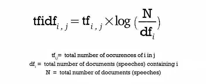
3.4-TF-IDF (Term Frequency-Inverse Document Frequency)

The TF-IDF score is the result of the multiplication of two values: term frequency and inverse document frequency.

Term Frequency: The number of times a term occurs in a document.

Inverse Document Frequency: Represents the rarity of a term by looking at all documents. The rarer the term, the higher the IDF score. If a term is present in all documents, the IDF is canceled out, as a term that appears everywhere has no importance in document classification.

Formula for TF-IDF:

3.5-Word2Vec

Word2Vec models, or word-to-vector models, were introduced by Tomas Mikolov et al. and are widely adopted for learning word embeddings or vector representations of words.

Word2Vec models internally use a simple neural network with a single layer and capture the weights of the hidden layer. The goal of training the model is to learn the weights of the hidden layer, which represent “word embeddings.” Although Word2Vec uses a neural network architecture, the architecture itself is not very complex and does not involve any non-linearity.

Word2Vec offers a range of models used to represent words in an n-dimensional space so that similar words and words with closer meanings are placed next to each other. Let’s review the two most commonly used models: Skip-Gram and Continuous Bag-of-Words (CBOW).

• **Skip-Gram: ** Skip-Gram predicts surrounding words using the current word in the sequence.

• **CBOW: ** In contrast to Skip-Gram, CBOW predicts the current word using the surrounding words in the sequence.

4-Machine Learning Models

After cleaning and vectorizing the data, we pass the vectors to a machine learning model for classification. We can use Naive Bayes algorithm as example.

Naive Bayes methods are supervised learning algorithms based on Bayes’ theorem. The term “Naive” corresponds to the independence assumption between the data to be classified.

Conclusion:

In conclusion, the journey through Natural Language Processing involves crucial stages: preprocessing to refine text, vectorization for numerical representation, and machine learning classification. Techniques like tokenization, cleaning, and vectorization methods such as One-Hot Encoding, Bag of Words, and Word2Vec play pivotal roles. The Naive Bayes algorithm stands out for classification. NLP’s impact continues to grow, reshaping industries and enhancing everyday experiences.