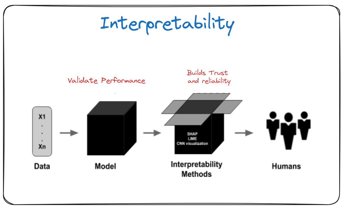
ML Explainability & Interpretability

Posted Nov 28, 2025 Updated Dec 13, 2025

By eya_garci 36 min read

Introduction

This article is a comprehensive and practical resource for mastering explainability and interpretability in Machine Learning. Designed for Data Scientists, ML Engineers, and AI Researchers, it covers:

✅ Solid Fundamentals - Key concepts, types of explanations
✅ Practical Methods - SHAP, LIME, PDP, ALE, Counterfactuals
✅ Informed Choices - Decision framework for choosing the right method
✅ Real-World Debugging - Solutions to common problems
✅ Causality - Difference between correlation vs causation
✅ Production-Ready - Architecture, APIs, monitoring
✅ Benchmarks - Quantitative performance comparisons
✅ Best Practices - Proven checklists and workflows

Objective

When and how to use each explainability method
Identify and resolve common problems (contradictory SHAP, unstable LIME, etc.)
Deploy to production performant explanations (< 100ms)
Understand the difference between correlational and causal explanations
Audit and mitigate biases in your models
Follow best practices from the industry

Learning Path Overview

📚 Fundamentals          🛠️ Practice              🚀 Expert
─────────────────────   ────────────────────    ─────────────────────
                                                  
Basic Concepts     →    Choose Method      →    Causal Inference
    ↓                        ↓                        ↓
Global vs Local    →    Debugging          →    Production Deploy
    ↓                        ↓                        ↓
Methods (SHAP,     →    Benchmarks         →    Monitoring & Scale
 LIME, PDP...)              ↓                        ↓
    ↓                   Best Practices      →    Complete Checklist
Advanced Techniques

Quick Start

Want quick answers?

“Which method to use?” → Choosing the Right Method
“My explanations are weird” → When Methods Fail
“How to deploy to production?” → Production Deployment
“How to audit fairness?” → Best Practices
“What’s the fastest method?” → Benchmarks

Fundamentals

Fundamental Concepts
- Definitions: Interpretability vs Explainability
- Model Types (Interpretable vs Black-Box)
Global vs Local Interpretability
- Global: Model overview
- Local: Individual prediction explanations

Methods & Techniques

Choosing the Right Method
- Decision Framework (decision tree)
- Quick decision matrix
- Red flags per method
- Recommended combinations
When Methods Fail
- SHAP: Contradictory values
- LIME: Extreme instability
- PDP: Misleading patterns
- Counterfactuals: Unrealistic suggestions
- Debugging checklist
Interpretation Methods
- SHAP (SHapley Additive exPlanations)
- LIME (Local Interpretable Model-agnostic Explanations)
- Permutation Importance
- Partial Dependence Plots (PDP)
- Individual Conditional Expectation (ICE)
- Accumulated Local Effects (ALE)
- Counterfactual Explanations

Advanced Concepts

Advanced Techniques
- Attention Mechanisms (Deep Learning)
- Saliency Maps (Vision)
- Anchors
- Prototypes & Criticisms
Causal vs Correlational Explanations
- The fundamental problem
- Correlation vs Causation
- Simpson’s Paradox in ML
- Causal Inference for ML
- Do-calculus, Propensity Score, Causal Forests

Performance & Production

Benchmarks & Comparisons
- Performance Comparison (latency, scalability)
- Accuracy & Fidelity Tests
- Stability Comparison
- Cost-Benefit Analysis
- Recommendation matrix
Production Deployment
- Architecture Overview
- Explainer as a Service (API)
- Performance optimizations
- Monitoring & Alerting
- Versioning & A/B Testing

Practical Resources

Tools & Implementation
- Python Libraries (SHAP, LIME, Fairlearn, etc.)
- Framework Comparison
- Recommended workflow
Best Practices
- Do’s and Don’ts
- Deployment checklist
Use Cases by Domain
- Healthcare
- Finance
- Justice
- E-commerce

Summary

Conclusion
- Golden rule
- Final checklist

Fundamental Concepts

Definitions

Interpretability: Ability to understand the model itself (intrinsically interpretable models)
Explainability: Ability to explain a model’s predictions (post-hoc)

Model Types

Intrinsically Interpretable Models:

Linear/logistic regression
Decision trees
Rules (IF-THEN)
GAM (Generalized Additive Models)

Black-Box Models:

Deep neural networks
Random Forests
XGBoost/LightGBM
SVM with complex kernels

Global vs Local Interpretability

Global Interpretability

Objective: Understand the model’s general behavior across the entire dataset

Characteristics:

Overall model overview
Identification of most important features
Understanding of general relationships

Examples:

Global feature importance
Permutation importance
Partial Dependence Plots (PDP)
Average feature effects

Local Interpretability

Objective: Explain a specific individual prediction

Characteristics:

Instance-by-instance explanation
Useful for critical decisions
May differ from global behavior

Examples:

SHAP values (local)
LIME
Individual Conditional Expectation (ICE)
Counterfactual explanations

Choosing the Right Method

Decision Framework

Step 1: Identify your needs

┌─ What type of explanation?
│  ├─ Global (general behavior) ────────────────┐
│  │  ├─ Feature importance? → Permutation Importance
│  │  ├─ Feature-target relationships? → PDP/ALE
│  │  └─ Complex interactions? → SHAP global
│  │
│  └─ Local (specific prediction) ────────────────┐
│     ├─ One critical instance? → SHAP/LIME
│     ├─ Actionable (what to change)? → Counterfactuals
│     └─ Simple rules? → Anchors
│
├─ What model type?
│  ├─ Tree-based (RF, XGBoost) → TreeSHAP (optimal)
│  ├─ Neural Network → Integrated Gradients / DeepSHAP
│  ├─ Linear → Coefficients + confidence intervals
│  └─ Model-agnostic required? → LIME / KernelSHAP
│
├─ Computational constraints?
│  ├─ Real-time (< 100ms)? → Pre-compute SHAP / Feature importance
│  ├─ Massive dataset? → TreeSHAP / Sampling
│  └─ Limited resources? → LIME (faster than SHAP)
│
└─ Correlated features?
   ├─ Yes, strongly → ALE > PDP
   └─ No → PDP (more intuitive)

Quick Decision Matrix

Need	Primary Method	Alternative	When to Avoid
Global feature importance	Permutation Importance	SHAP global	Highly correlated features
Feature effect	ALE (if correlations)	PDP	Dangerous extrapolation
Reliable local explanation	SHAP	LIME	Strict real-time
Fast explanation	LIME	Linear surrogate	High precision required
Actionable	Counterfactuals	Anchors	Impossible changes
Maximum interpretability	Anchors	Decision rules	Low coverage acceptable
Deep Learning (vision)	Grad-CAM	Integrated Gradients	Non-CNN model
Deep Learning (NLP)	Attention weights	LIME text	Attention not available

Red Flags per Method

Do NOT use SHAP if:

Real-time deadline < 50ms and complex model
Dataset > 1M instances without sampling
Unsupported model (custom SHAP implementation takes long)

Do NOT use LIME if:

Reproducibility is critical (unstable results)
Explanation must be exact (approximation)
Many categorical features (difficult perturbation)

Do NOT use PDP if:

Strongly correlated features (use ALE instead)
Dominant interactions (masked by averaging)
Extrapolation outside distribution

Do NOT use Counterfactuals if:

User cannot modify features (age, history)
Feasibility not verifiable
Multiple simultaneous changes impossible

Recommended Combinations

Standard Workflow (Production)

  
# 1. Global understanding
perm_importance = permutation_importance(model, X_val, y_val)
top_features = get_top_k(perm_importance, k=10)

# 2. Feature relationships (for top features)
for feat in top_features:
    if is_correlated(feat, other_features):
        plot_ale(model, X_train, feat)  # Robust to correlation
    else:
        plot_pdp(model, X_train, feat)  # More intuitive

# 3. Local explanations (for critical decisions)
explainer = shap.TreeExplainer(model)  # Pre-compute
shap_values = explainer(X_critical)

Complete Audit (Pre-deployment)

  
# Global
- Permutation importance
- SHAP global summary
- ALE/PDP for top 5 features
- Feature interactions (H-statistic)

# Local
- SHAP for 100 random instances
- LIME comparison (verify consistency)
- Counterfactuals for edge cases

# Validation
- Stability test (re-run, check variance)
- Domain expert review
- Fairness audit by subgroups

When Methods Fail

Common Failure Scenarios

1. SHAP: Contradictory Values

Symptom: SHAP says feature X is positively important, but increasing X decreases prediction

Causes:

Complex non-linear interactions: SHAP shows marginal contribution, not total effect
Correlated features: SHAP arbitrarily shares effect between correlated features
Extrapolation: KernelSHAP creates out-of-distribution instances

Solution:

  
# Check interactions
shap.dependence_plot("feature_X", shap_values, X_test, interaction_index="auto")

# Analyze correlations
import seaborn as sns
sns.heatmap(X_train.corr(), annot=True)

# If correlation > 0.7: group features
from sklearn.decomposition import PCA
X_pca = PCA(n_components=10).fit_transform(X_train)

Real Example:

# Feature: "income" and "zip_code" correlated (wealthy neighborhoods)
# SHAP may attribute effect to one or the other unstably
# Solution: create composite feature "socioeconomic_profile"

2. LIME: Extreme Instability

Symptom: Re-running LIME gives radically different explanations

Causes:

Poorly chosen neighborhood: Perturbations leave the distribution
Strong local non-linearity: Linear model cannot approximate
Random seed: Stochastic sampling

Diagnosis:

  
# Stability test
explanations = []
for seed in range(10):
    exp = explainer.explain_instance(
        X_test[0], 
        model.predict_proba,
        num_samples=5000,  # Increase!
        random_state=seed
    )
    explanations.append(exp.as_list())

# Calculate coefficient variance
import numpy as np
coef_variance = np.var([e[0][1] for e in explanations])
if coef_variance > 0.1:  # Arbitrary threshold
    print("⚠️ LIME unstable, use SHAP")

Solutions:

  
# 1. Increase num_samples (5000+)
# 2. Set appropriate kernel_width
explainer = lime_tabular.LimeTabularExplainer(
    X_train,
    kernel_width=np.sqrt(X_train.shape[1]) * 0.75,  # Empirical rule
    sample_around_instance=True
)

# 3. Average over multiple runs
from collections import defaultdict
coefs = defaultdict(list)
for _ in range(20):
    exp = explainer.explain_instance(...)
    for feat, coef in exp.as_list():
        coefs[feat].append(coef)
        
average_coefs = {k: np.mean(v) for k, v in coefs.items()}

3. PDP: Misleading Patterns

Symptom: PDP shows linear relationship but model is non-linear

Causes:

Averaging effect: Masks underlying heterogeneities
Correlated features: Creates unrealistic instances
Extrapolation: Regions of space never seen in training

Detection:

  
from sklearn.inspection import PartialDependenceDisplay

# Compare PDP (average) vs ICE (individual)
fig, (ax1, ax2) = plt.subplots(1, 2, figsize=(12, 4))

PartialDependenceDisplay.from_estimator(
    model, X_train, ["age"], 
    kind="average", ax=ax1
)  # PDP

PartialDependenceDisplay.from_estimator(
    model, X_train, ["age"], 
    kind="both", ax=ax2
)  # ICE + PDP

# If ICE curves diverge strongly → hidden heterogeneity

Solution - Use ALE:

  
from alepython import ale

# ALE handles correlations better
ale_eff = ale(
    X=X_train.values, 
    model=model.predict, 
    feature=[feature_idx],
    grid_size=50
)

4. Counterfactuals: Unrealistic Suggestions

Symptom: “To be approved, increase your age by 15 years”

Causes:

No feasibility constraints
Optimization finds bizarre local minimum
Immutable features not specified

Solution:

  
import dice_ml

# Specify immutable features
immutable_features = ['age', 'gender', 'past_credit_history']

# Plausibility constraints
feature_ranges = {
    'income': (10000, 200000),  # Realistic limits
    'debt_ratio': (0, 1),
    'nb_credits': (0, 10)
}

exp = dice_ml.Dice(d, m, method='genetic')  # More robust method
cf = exp.generate_counterfactuals(
    query_instance=X_test[0:1],
    total_CFs=5,
    desired_class='opposite',
    permitted_range=feature_ranges,
    features_to_vary=[f for f in feature_names if f not in immutable_features],
    diversity_weight=0.5  # Generate diverse CFs
)

# Verify plausibility
for cf_instance in cf.cf_examples_list[0].final_cfs_df.values:
    if not is_plausible(cf_instance, X_train):
        print(f"⚠️ CF out of distribution: {cf_instance}")

5. Permutation Importance: Surprising Results

Symptom: “Important” feature according to model has permutation importance = 0

Causes:

Redundant features: Other feature compensates
Overfitting: Spurious importance in training, not in test
Random variations: Not enough n_repeats

Diagnosis:

  
from sklearn.inspection import permutation_importance

# Test on train vs test
perm_train = permutation_importance(
    model, X_train, y_train, 
    n_repeats=30, 
    random_state=42
)
perm_test = permutation_importance(
    model, X_test, y_test, 
    n_repeats=30, 
    random_state=42
)

# Compare
import pandas as pd
comparison = pd.DataFrame({
    'feature': feature_names,
    'importance_train': perm_train.importances_mean,
    'importance_test': perm_test.importances_mean,
    'diff': perm_train.importances_mean - perm_test.importances_mean
})

# If diff > 0.05 → overfitting on this feature
overfit_features = comparison[comparison['diff'] > 0.05]
print(f"⚠️ Overfitting features: {overfit_features['feature'].tolist()}")

Solution:

  
# Detect redundancy
from sklearn.feature_selection import SelectKBest, f_classif
from scipy.stats import spearmanr

# Spearman correlation matrix (robust to non-linear)
corr_matrix = X_train.corr(method='spearman')

# Identify correlated pairs
high_corr_pairs = []
for i in range(len(corr_matrix.columns)):
    for j in range(i+1, len(corr_matrix.columns)):
        if abs(corr_matrix.iloc[i, j]) > 0.8:
            high_corr_pairs.append((
                corr_matrix.columns[i], 
                corr_matrix.columns[j],
                corr_matrix.iloc[i, j]
            ))

print(f"Redundant features: {high_corr_pairs}")
# → Remove one or create composite feature

Debugging Checklist

When an explanation seems wrong:

  
# 1. Verify the model itself
assert model.score(X_test, y_test) > 0.7, "Poorly performing model"

# 2. Check data leakage
from sklearn.inspection import permutation_importance
perm = permutation_importance(model, X_test, y_test)
if perm.importances_mean.max() > 0.9:
    print("⚠️ Possible data leakage")

# 3. Test multiple methods (triangulation)
shap_importance = np.abs(shap_values).mean(0)
lime_importance = get_lime_importance(model, X_test)
perm_importance = permutation_importance(model, X_test, y_test).importances_mean

# If correlation between methods < 0.5 → investigation needed
from scipy.stats import spearmanr
shap_lime_corr = spearmanr(shap_importance, lime_importance).correlation
if shap_lime_corr < 0.5:
    print("⚠️ Methods don't agree, investigate")

# 4. Validate with domain expert
# If explanation contradicts business knowledge → likely bug

# 5. Test on synthetic instances
# Create case where answer is known
X_synthetic = create_test_case(feature_X=high_value, others=baseline)
pred = model.predict(X_synthetic)
explanation = explainer.explain(X_synthetic)
assert explanation['feature_X'] > 0, "Inconsistent explanation"

General Remedies

Problem: Unstable explanations

Increase samples (LIME: num_samples=5000+)
Average over multiple runs
Use more stable method (SHAP > LIME)

Problem: Counter-intuitive explanations

Check correlated features (ALE > PDP)
Check interactions (dependence plots)
Validate with domain expert

Problem: Degraded performance

Pre-compute explainers
Strategic sampling
Approximations (TreeSHAP vs KernelSHAP)

Problem: Non-actionable explanations

Use counterfactuals with constraints
Specify immutable features
Verify plausibility vs training distribution

Interpretation Methods

1. SHAP (SHapley Additive exPlanations)

Principle: Based on game theory (Shapley values)

📐 Mathematical Foundations

Simple Definition: A feature’s SHAP value measures its contribution by considering all possible combinations of other features.

How it works:

For each feature, test its impact in all possible subsets of other features
Calculate the difference in prediction with and without this feature
Take a weighted average of these differences
Weight depends on subset size

Intuition: It’s like asking “what is this feature’s average contribution across all possible contexts?”

Guaranteed Axioms (Shapley properties):

Efficiency (Additivity):
- Sum of all SHAP contributions = final prediction
- base_value + contribution_feature1 + contribution_feature2 + … = prediction
Symmetry:
- If two features contribute identically in all contexts, they have the same SHAP value
Dummy:
- A feature that never changes the prediction has SHAP value = 0
Additivity:
- For an ensemble of models, SHAP remains additive

Why It’s Important: These axioms guarantee that SHAP is fair and mathematically consistent.

Advantages:

✅ Solid theoretical foundation (only method with formal guarantees)
✅ Guaranteed mathematical properties (additivity, symmetry, dummy)
✅ Global + Local
✅ Consistent and fair
✅ Automatically captures interactions

Limitations:

❌ Computationally expensive: $O(2^M)$ coalitions (M features)
❌ Can be slow on large datasets without approximation
❌ KernelSHAP creates out-of-distribution instances (correlated features)
❌ Causal interpretation not always correct

Variants:

TreeSHAP: Optimized for trees (XGBoost, Random Forest)
KernelSHAP: Model-agnostic
DeepSHAP: For neural networks
LinearSHAP: For linear models

  
import shap

# TreeSHAP for XGBoost
explainer = shap.TreeExplainer(model)
shap_values = explainer.shap_values(X_test)

# Visualizations
shap.summary_plot(shap_values, X_test)  # Global
shap.waterfall_plot(shap_values[0])     # Local
shap.dependence_plot("feature_name", shap_values, X_test)

Interpretation:

Positive value: feature pushes toward positive class
Negative value: feature pushes toward negative class
Magnitude: importance of contribution

2. LIME (Local Interpretable Model-agnostic Explanations)

Principle: Locally approximates the complex model with a simple linear model

Process:

Perturb the instance around the point of interest
Obtain predictions from the black-box model
Train a weighted local linear model

Advantages:

✅ Model-agnostic
✅ Intuitive (linear coefficients)
✅ Supports text, images, tabular

Limitations:

❌ Instability (results can vary)
❌ Neighborhood choice critical
❌ No strong theoretical guarantees

  
from lime import lime_tabular

explainer = lime_tabular.LimeTabularExplainer(
    X_train,
    feature_names=feature_names,
    class_names=class_names,
    mode='classification'
)

explanation = explainer.explain_instance(
    X_test[0], 
    model.predict_proba,
    num_features=10
)
explanation.show_in_notebook()

3. Permutation Importance

Principle: Measures performance degradation when a feature is permuted (noised)

Algorithm:

Calculate baseline metric on unmodified data
For each feature:
- Randomly permute its values
- Recalculate the metric
- Importance = performance degradation
Repeat and average for stability

Advantages:

✅ Model-agnostic
✅ Simple to understand
✅ Captures interactions
✅ Reflects real importance for the task

Limitations:

❌ Expensive (requires multiple re-evaluations)
❌ Sensitive to correlated features
❌ Can create unrealistic instances

  
from sklearn.inspection import permutation_importance

perm_importance = permutation_importance(
    model, X_test, y_test,
    n_repeats=10,
    random_state=42,
    scoring='accuracy'
)

# Visualization
import pandas as pd
importance_df = pd.DataFrame({
    'feature': feature_names,
    'importance': perm_importance.importances_mean,
    'std': perm_importance.importances_std
}).sort_values('importance', ascending=False)

4. Partial Dependence Plots (PDP)

Principle: Shows the marginal average effect of one/two feature(s) on the prediction

How it works:

Fix the feature of interest at a specific value
Vary all other features according to their values in the dataset
Calculate the average prediction
Repeat for different values of the feature of interest
Simplified formula: Average of predictions for a given feature value

Advantages:

✅ Clear visualization of relationship
✅ Model-agnostic
✅ Supports 1D and 2D

Limitations:

❌ Assumes feature independence (problem if correlation)
❌ Can mask heterogeneities (averaging effect)
❌ Expensive for continuous features

  
from sklearn.inspection import PartialDependenceDisplay

features = [0, 1, (0, 1)]  # 2 1D features + 1 2D interaction
PartialDependenceDisplay.from_estimator(
    model, X_train, features,
    feature_names=feature_names
)

5. Individual Conditional Expectation (ICE)

Principle: Disaggregated version of PDP - shows effect for each instance individually

Difference with PDP:

PDP = average of ICE curves
ICE shows heterogeneity of effects

Advantages:

✅ Reveals complex interactions
✅ Detects subgroups with different behaviors
✅ Doesn’t mask heterogeneity

Limitations:

❌ Difficult to read with many instances
❌ Assumes feature independence

  
from sklearn.inspection import PartialDependenceDisplay

display = PartialDependenceDisplay.from_estimator(
    model, X_train, [0],
    kind='individual',  # ICE curves
    feature_names=feature_names
)

# Combine ICE + PDP
display = PartialDependenceDisplay.from_estimator(
    model, X_train, [0],
    kind='both',  # ICE + PDP average
    feature_names=feature_names
)

6. Accumulated Local Effects (ALE)

Principle: Alternative to PDP that handles correlated features better

Difference with PDP:

PDP: varies feature across entire range (creates unrealistic instances if correlation)
ALE: accumulates local effects in small intervals (stays in dense regions)

Advantages:

✅ Robust to correlated features
✅ No extrapolation in unrealistic zones
✅ More reliable causal interpretation
✅ Faster than PDP

Mathematical principle:

ALE accumulates local changes in prediction
Instead of global averaging (PDP), sum effects in small intervals
This avoids extrapolating in non-existent data regions

  
from alepython import ale

# Installation: pip install alepython
ale_eff = ale(
    X=X_train,
    model=model,
    feature=[0],  # feature index
    grid_size=50
)

7. Counterfactual Explanations

Principle: “What would need to change minimally to obtain a different prediction?”

Objective: Find $x’$ close to $x$ such that $f(x’) \neq f(x)$

Optimization objective: Find minimal change that flips prediction by balancing:

Proximity: Stay close to original instance (minimal distance)
Effectiveness: Reach desired target class (minimize error)
Realism: Stay in plausible regions (regularization)

Advantages:

✅ Actionable (says “what to change”)
✅ Intuitive for non-technical users
✅ Useful for recourse/appeal

Limitations:

❌ Can suggest unrealistic changes
❌ Non-uniqueness (multiple counterfactuals possible)
❌ Computational cost

  
import dice_ml

# Setup
d = dice_ml.Data(dataframe=df, continuous_features=cont_cols, outcome_name='target')
m = dice_ml.Model(model=model, backend='sklearn')
exp = dice_ml.Dice(d, m, method='random')

# Generate counterfactuals
cf = exp.generate_counterfactuals(
    query_instance=X_test[0:1],
    total_CFs=3,  # number of counterfactuals
    desired_class='opposite'
)
cf.visualize_as_dataframe()

Popular methods:

DiCE (Diverse Counterfactual Explanations)
FACE (Feasible and Actionable)
WachterCF (Wachter et al.)
Anchors

Advanced Techniques

Attention Mechanisms (Deep Learning)

Principle: Visualize where the model “looks”

Applications:

NLP: which words are important
Vision: which image regions
Time series: which timesteps

  
# Example with transformers
from transformers import pipeline

classifier = pipeline("sentiment-analysis", return_all_scores=True)
result = classifier("This movie is amazing!", return_attention=True)
# Visualize attention weights

Saliency Maps (Vision)

Techniques:

Gradient-based: Grad-CAM, Integrated Gradients
Perturbation-based: Occlusion sensitivity
CAM/Grad-CAM: Class Activation Mapping

  
import torch
from pytorch_grad_cam import GradCAM

model = torchvision.models.resnet50(pretrained=True)
target_layers = [model.layer4[-1]]
cam = GradCAM(model=model, target_layers=target_layers)

grayscale_cam = cam(input_tensor=image, targets=None)

Anchors

Principle: IF-THEN rules that guarantee a prediction with high precision

Example:

IF age > 45 AND income > 50k THEN approved (95% precision)

Advantages:

✅ Highly interpretable (simple rules)
✅ Locally guaranteed precision
✅ Explicit coverage

Prototypes & Criticisms

Principle:

Prototypes: representative examples of each class
Criticisms: examples poorly represented by prototypes

Methods:

MMD-critic
ProtoDash
Influence functions

Causal vs Correlational Explanations

The Fundamental Problem

SHAP, LIME, PDP are NOT causal - they show associations, not causation

Classic Example:

# Model predicts lung cancer probability
# SHAP says: feature 'yellow fingers' very important
# But: yellow fingers are CORRELATED (smoking), not CAUSAL
# Bleaching fingers doesn't reduce cancer!

Correlation vs Causation

Aspect	Correlational Explanation	Causal Explanation
Question	Which features are associated with the prediction?	Which features cause the prediction?
Method	SHAP, LIME, PDP	Causal inference, do-calculus
Intervention	“If feature X were different”	“If we change feature X”
Validity	Passive observation	Active intervention
Actionable	⚠️ Can be misleading	✅ Truly actionable

Simpson’s Paradox in ML

Real Example:

  
# University admission dataset
# SHAP says: "male gender increases admission"
# BUT controlling for department:
#   - Men apply to competitive departments (CS, engineering)
#   - Women apply to less competitive departments (humanities)
# True cause: department, not gender!

# Correlational explanation (SHAP)
shap_values['gender_male']  # Positive (+0.3)

# Causal explanation (after adjustment)
from econml.dml import CausalForestDML
causal_effect = model.effect(X, treatment='gender_male')
print(causal_effect)  # Close to 0 or negative!

When Correlation ≈ Causation?

Necessary conditions:

No confounding: No hidden variable causing both X and Y
No reverse causality: Y does not cause X
No selection bias: Unbiased sampling

In practice: Rarely satisfied!

🛑 Causal Inference for ML Explanations

1. Causal Discovery

Identify causal structure of features

  
from causallearn.search.ConstraintBased.PC import pc
from causallearn.utils.cit import chisq

# Discover causal graph
cg = pc(
    data=X_train.values,
    alpha=0.05,  # Significance level
    indep_test=chisq
)

# Visualize
from causallearn.utils.GraphUtils import GraphUtils
GraphUtils.to_pydot(cg.G).write_png('causal_graph.png')

# Identify confounders
confounders = find_confounders(cg.G, treatment='X', outcome='Y')
print(f"Adjust for: {confounders}")

2. Do-Calculus for Interventions

Notation:

P(Y X=x) = observation: “Y when we observe X=x”
P(Y do(X=x)) = intervention: “Y when we set X=x”

Key difference:

# Observational: SHAP/LIME
# We observe X=x naturally, Z can be correlated with X
# Expectation of Y given X=x, averaging over conditional distribution of Z given X

# Interventional: Causal
# We force X=x (intervention), Z remains according to its natural distribution
# Expectation of Y given we set X=x, averaging over marginal distribution of Z
# Difference: P(Z) no longer depends on X!

Implementation:

  
import dowhy
from dowhy import CausalModel

# Define causal model
model = CausalModel(
    data=df,
    treatment='feature_X',
    outcome='prediction',
    common_causes=['confounder_1', 'confounder_2'],
    instruments=['instrumental_var']  # If available
)

# Identify causal effect
identified_estimand = model.identify_effect(
    proceed_when_unidentifiable=True
)

# Estimate
estimate = model.estimate_effect(
    identified_estimand,
    method_name="backdoor.propensity_score_weighting"
)

print(f"Causal effect: {estimate.value}")
print(f"Confidence interval: {estimate.get_confidence_intervals()}")

# Refutation tests
refute = model.refute_estimate(
    identified_estimand, 
    estimate,
    method_name="random_common_cause"
)
print(refute)

3. Propensity Score Matching

Create comparable groups to estimate causal effect

  
from sklearn.linear_model import LogisticRegression
from sklearn.neighbors import NearestNeighbors

# 1. Estimate propensity score P(Treatment=1 | X)
propensity_model = LogisticRegression()
propensity_model.fit(X_covariates, treatment)
propensity_scores = propensity_model.predict_proba(X_covariates)[:, 1]

# 2. Matching
treated_idx = np.where(treatment == 1)[0]
control_idx = np.where(treatment == 0)[0]

nn = NearestNeighbors(n_neighbors=1, metric='euclidean')
nn.fit(propensity_scores[control_idx].reshape(-1, 1))
matches = nn.kneighbors(
    propensity_scores[treated_idx].reshape(-1, 1),
    return_distance=False
)

# 3. Calculate causal effect (ATE)
matched_control_idx = control_idx[matches.flatten()]
ate = (
    y_outcome[treated_idx].mean() 
    - y_outcome[matched_control_idx].mean()
)

print(f"Average Treatment Effect: {ate:.3f}")

4. Causal Forests

Estimate heterogeneous causal effects (varies by instance)

  
from econml.dml import CausalForestDML
from sklearn.ensemble import RandomForestRegressor

# Model
causal_forest = CausalForestDML(
    model_y=RandomForestRegressor(),  # Model for Y
    model_t=RandomForestRegressor(),  # Model for treatment
    n_estimators=1000,
    min_samples_leaf=10
)

# Fit
causal_forest.fit(
    Y=y_outcome,
    T=treatment,
    X=X_features,
    W=X_confounders  # Confounders
)

# Individual causal effect (CATE)
cate = causal_forest.effect(X_test)

# Interpretation: "For this person, treating increases outcome by X"
print(f"CATE for instance 0: {cate[0]:.3f}")

# Causal feature importance
from econml.sklearn_extensions.model_selection import GridSearchCVList
shap_values_causal = causal_forest.shap_values(X_test)
# These SHAP values are causal because the model is causal!

Practical Guidelines

When to Use Correlational Explanations (SHAP/LIME)?

✅ OK for:

Debugging: Understand what the model learned
Fairness audit: Detect bias
Compliance: Explain decision (“why this score?”)
Feature engineering: Identify informative features

❌ NOT OK for:

Actionable recommendations: “Change X to improve Y”
Policy decisions: Decide on interventions
Causal claims: “X causes Y”
Realistic counterfactuals: “If you had done X…”

When to Use Causal Explanations?

✅ Required for:

Interventions: Recommend actions
What-if scenarios: Simulate changes
A/B testing planning: Predict effect of interventions
Fairness mitigation: Identify true causes of bias
Regulatory compliance: Some domains require causality

Hybrid Workflow

  
# Phase 1: Exploration (correlational)
shap_values = explainer.shap_values(X)
top_features = get_top_features(shap_values, k=10)

# Phase 2: Causal validation
for feature in top_features:
    # Test if correlation is causal
    causal_effect = estimate_causal_effect(
        data=df,
        treatment=feature,
        outcome='target',
        confounders=other_features
    )
    
    if abs(causal_effect) > threshold:
        print(f"✅ {feature} is causal")
        # Use for recommendations
    else:
        print(f"⚠️ {feature} correlated but non-causal")
        # Don't recommend changing

# Phase 3: Action
# Only recommend changing causal features
actionable_features = [f for f in top_features if is_causal(f)]
generate_recommendations(actionable_features)

Key Takeaways

SHAP/LIME/PDP answer: “Which features does the model use?”
Causal inference answers: “What would happen if we change X?”
For model debugging: Correlational OK
For recommendations: Causal required
Always be explicit: “This is an association, not necessarily causal”

Causal Inference Resources

Book: “Causal Inference in Statistics: A Primer” - Pearl, Glymour, Jewell
Book: “The Book of Why” - Judea Pearl
Library: DoWhy (Microsoft), EconML (Microsoft), CausalML (Uber)
Paper: “Causal Interpretability for Machine Learning” - Moraffah et al. (2020)

Benchmarks & Comparisons

Performance Comparison

Types of bias:

Historical bias: Data reflects past discrimination
Representation bias: Some groups under-represented
Measurement bias: Imperfect proxy variables
Aggregation bias: One model for all doesn’t fit anyone
Evaluation bias: Metrics don’t capture all aspects

Detection:

  
# Analyze distribution by group
df.groupby('protected_attribute')['target'].mean()

# Disparate impact
from aif360.metrics import BinaryLabelDatasetMetric
metric = BinaryLabelDatasetMetric(dataset, 
    unprivileged_groups=[{'sex': 0}],
    privileged_groups=[{'sex': 1}])
print(metric.disparate_impact())

Fairness Metrics

Choosing the Right Fairness Criterion

Decision Tree for Fairness Metric Selection:

┌─ What is the context?
│
├─ 🏥 Healthcare / Safety-Critical
│  └─> Use: Equalized Odds or Equal Opportunity
│      Rationale: Same quality of care for all groups
│      Example: Cancer detection should have equal TPR
│
├─ 💰 Finance / Lending
│  ├─ Focus on acceptance rates?
│  │  └─> Use: Demographic Parity
│  │      Rationale: Equal opportunity to access credit
│  └─ Focus on loan quality?
│     └─> Use: Calibration
│         Rationale: Predicted risk should match actual risk
│
├─ ⚖️ Criminal Justice
│  └─> Use: Equalized Odds + Calibration
│      Rationale: Mistakes equally distributed + probabilities meaningful
│      Example: Recidivism prediction
│
├─ 🎓 Education / Hiring
│  └─> Use: Equal Opportunity
│      Rationale: Qualified candidates should have equal chance
│      Example: Interview callback rates
│
└─ 🛒 E-commerce / Advertising
   └─> Use: Demographic Parity (lower priority)
       Rationale: Exposure to opportunities
       Example: Job ads shown equally

Fairness Metrics Explained

1. Demographic Parity (Statistical Parity)

Formula in text: Probability of positive prediction is the same for all groups

P(prediction=1 group A) = P(prediction=1 group B)

Definition: Equal positive prediction rate between groups

When to use:

✅ Equal access important (lending, hiring)
✅ Combatting historical discrimination
✅ Marketing/advertising fairness

Limitations:

❌ Ignores base rates (groups may have different true positive rates)
❌ Can hurt accuracy
❌ May violate individual fairness

Implementation:

  
# Ratio: value close to 1 = fair
selection_rate_group0 = predictions[group_0].mean()
selection_rate_group1 = predictions[group_1].mean()
demographic_parity_ratio = selection_rate_group0 / selection_rate_group1

# Rule of thumb: 0.8 < ratio < 1.25 is acceptable
if 0.8 <= demographic_parity_ratio <= 1.25:
    print("✅ Passes demographic parity")
else:
    print(f"⚠️ Fails demographic parity: {demographic_parity_ratio:.2f}")

Example:

Loan Approval:
- Group A: 40% approved
- Group B: 30% approved
- Ratio: 0.75 ❌ Fails (< 0.8)
→ Potential disparate impact

2. Equalized Odds

Formula in text: For each true class (positive and negative), positive prediction rate is the same for all groups

P(prediction=1 true_class=1, group A) = P(prediction=1 true_class=1, group B)
P(prediction=1 true_class=0, group A) = P(prediction=1 true_class=0, group B)

Definition: TPR (True Positive Rate) AND FPR (False Positive Rate) equal between groups

When to use:

✅ Healthcare (equal treatment quality)
✅ Criminal justice (equal error rates)
✅ High-stakes decisions

Advantage: Stronger than demographic parity (accounts for ground truth)

Implementation:

  
from sklearn.metrics import confusion_matrix

def calculate_equalized_odds(y_true, y_pred, sensitive):
    """Calculate TPR and FPR gap between groups"""
    groups = sensitive.unique()
    metrics = {}
    
    for group in groups:
        mask = (sensitive == group)
        tn, fp, fn, tp = confusion_matrix(
            y_true[mask], 
            y_pred[mask]
        ).ravel()
        
        tpr = tp / (tp + fn) if (tp + fn) > 0 else 0
        fpr = fp / (fp + tn) if (fp + tn) > 0 else 0
        
        metrics[group] = {'tpr': tpr, 'fpr': fpr}
    
    # Calculate differences
    tpr_diff = abs(metrics[groups[0]]['tpr'] - metrics[groups[1]]['tpr'])
    fpr_diff = abs(metrics[groups[0]]['fpr'] - metrics[groups[1]]['fpr'])
    
    print(f"TPR difference: {tpr_diff:.3f}")
    print(f"FPR difference: {fpr_diff:.3f}")
    
    # Passes if both < 0.1 (rule of thumb)
    passes = (tpr_diff < 0.1) and (fpr_diff < 0.1)
    return passes, metrics

# Usage
calculate_equalized_odds(y_test, y_pred, sensitive_features)

Example (Medical Diagnosis):

Disease Detection:
Group A: TPR=0.85, FPR=0.10
Group B: TPR=0.75, FPR=0.15

TPR diff = 0.10 ❌ (group B misses more cases)
FPR diff = 0.05 ✅
→ Fails equalized odds (unequal treatment quality)

3. Equal Opportunity

Formula in text: Among true positives, positive prediction rate is the same for all groups

P(prediction=1 true_class=1, group A) = P(prediction=1 true_class=1, group B)

Definition: TPR (True Positive Rate) equal between groups (relaxation of equalized odds)

When to use:

✅ When false positives less critical than false negatives
✅ Hiring (qualified candidates equal chance)
✅ College admission

Rationale: Focus on “qualified positives” getting equal treatment

Implementation:

  
from sklearn.metrics import recall_score

# Only check TPR (not FPR)
tpr_group0 = recall_score(y_true[group_0], y_pred[group_0])
tpr_group1 = recall_score(y_true[group_1], y_pred[group_1])
tpr_diff = abs(tpr_group0 - tpr_group1)

print(f"TPR Group 0: {tpr_group0:.3f}")
print(f"TPR Group 1: {tpr_group1:.3f}")
print(f"Difference: {tpr_diff:.3f}")

if tpr_diff < 0.1:
    print("✅ Passes equal opportunity")

4. Predictive Parity

Formula in text: Among those predicted positive, proportion of true positives is the same for all groups

P(true_class=1 prediction=1, group A) = P(true_class=1 prediction=1, group B)

Definition: Precision (Positive Predictive Value) equal between groups

When to use:

✅ When false positives very costly
✅ Resource allocation
✅ Fraud detection

Interpretation: “If predicted positive, probability of actually being positive is equal”

Implementation:

  
from sklearn.metrics import precision_score

ppv_group0 = precision_score(y_true[group_0], y_pred[group_0])
ppv_group1 = precision_score(y_true[group_1], y_pred[group_1])

print(f"Precision Group 0: {ppv_group0:.3f}")
print(f"Precision Group 1: {ppv_group1:.3f}")

5. Calibration

Formula in text: For each predicted probability level, actual proportion of positives is the same for all groups

P(true_class=1 predicted_prob=p, group A) = P(true_class=1 predicted_prob=p, group B)

Definition: Predicted probabilities well calibrated by group

When to use:

✅ Probabilistic predictions important
✅ Risk assessment
✅ Medical prognosis

Implementation:

  
from sklearn.calibration import calibration_curve

for group in groups:
    mask = (sensitive == group)
    prob_true, prob_pred = calibration_curve(
        y_true[mask],
        y_pred_proba[mask],
        n_bins=10
    )
    
    plt.plot(prob_pred, prob_true, marker='o', label=f'Group {group}')

plt.plot([0, 1], [0, 1], linestyle='--', label='Perfect calibration')
plt.xlabel('Predicted probability')
plt.ylabel('True probability')
plt.legend()

Example: If model predicts 70% risk, actual outcome should be 70% for ALL groups

Impossibility Results

Theorem (Chouldechova 2017): If base rates differ between groups - meaning the actual proportion of positives is not the same in each group - then we CANNOT simultaneously satisfy:

Calibration (accurate probabilities)
Equalized Odds or Equal Opportunity (balanced errors)

Theorem (Kleinberg et al. 2016): We cannot simultaneously have:

Calibration
Balance for positive class
Balance for negative class

Practical Implication: We must choose which fairness definition to prioritize based on context!

Trade-off Example:

  
# Scenario: Different base rates
# Group A: 20% positive rate
# Group B: 40% positive rate

# If we want Demographic Parity (equal acceptance):
# → Will necessarily violate calibration or equalized odds

# If we want Calibration (accurate probabilities):
# → Acceptance rates will differ

# CHOICE REQUIRED based on values and context!

Practical Fairness Workflow

  
def comprehensive_fairness_audit(model, X, y, sensitive_attr):
    """
    Comprehensive fairness audit with multiple metrics
    """
    y_pred = model.predict(X)
    y_pred_proba = model.predict_proba(X)[:, 1]
    
    results = {}
    # [Implementation continues...]

Fairness Mitigation

Pre-processing:

Reweighting
Disparate impact remover
Resampling

In-processing:

Adversarial debiasing
Prejudice remover
Fair classification algorithms

Post-processing:

Calibrated equalized odds
Reject option classification
Threshold optimization per group

  
from aif360.algorithms.preprocessing import Reweighing
from aif360.algorithms.inprocessing import AdversarialDebiasing
from aif360.algorithms.postprocessing import CalibratedEqOddsPostprocessing

# Pre-processing
rw = Reweighing(unprivileged_groups=unprivileged_groups,
                privileged_groups=privileged_groups)
dataset_transf = rw.fit_transform(dataset)

# In-processing
debiaser = AdversarialDebiasing(
    unprivileged_groups=unprivileged_groups,
    privileged_groups=privileged_groups,
    scope_name='debiased_classifier',
    debias=True
)
debiaser.fit(dataset)

# Post-processing
cpp = CalibratedEqOddsPostprocessing(
    unprivileged_groups=unprivileged_groups,
    privileged_groups=privileged_groups
)
dataset_transf_pred = cpp.fit_predict(dataset, dataset_pred)

Trade-offs

Impossibility Theorems:

We cannot satisfy all fairness definitions simultaneously
Trade-off between fairness and accuracy
Choice depends on context and values

Example: A model can be fair according to demographic parity but unfair according to equalized odds

Model Cards & Documentation

Key elements:

Model Details: Architecture, training
Intended Use: Intended and excluded use cases
Factors: Variables, demographic groups
Metrics: Overall performance and by subgroup
Training/Evaluation Data: Provenance, known biases
Ethical Considerations: Risks, limitations
Recommendations: Best practices for use

  
# Model Card Template
model_card = {
    "model_details": {
        "name": "Credit Scoring Model",
        "version": "1.0",
        "date": "2025-11-28",
        "type": "XGBoost Classifier"
    },
    "intended_use": {
        "primary": "Predict loan default risk",
        "out_of_scope": "Not for criminal justice"
    },
    "factors": {
        "relevant": ["income", "credit_history", "age"],
        "evaluation_factors": ["gender", "ethnicity"]
    },
    "metrics": {
        "overall": {"accuracy": 0.85, "auc": 0.90},
        "by_group": {
            "male": {"accuracy": 0.86, "auc": 0.91},
            "female": {"accuracy": 0.84, "auc": 0.89}
        }
    },
    "ethical_considerations": [
        "Historical bias in loan approval data",
        "Disparate impact on protected groups"
    ]
}

Tools & Implementation

Python Libraries

Interpretability

  
pip install shap lime eli5 interpret
pip install scikit-learn>=1.0  # For PDP, permutation importance
pip install alepython  # For ALE plots
pip install dice-ml  # For counterfactuals

Fairness

  
pip install aif360  # IBM AI Fairness 360
pip install fairlearn  # Microsoft Fairlearn
pip install themis-ml

Visualization

  
pip install matplotlib seaborn plotly
pip install dtreeviz  # Visualize decision trees

Framework Comparison

Framework	Global	Local	Model-Agnostic	Fairness	Deep Learning
SHAP	✅	✅	✅	❌	✅ (DeepSHAP)
LIME	❌	✅	✅	❌	✅
InterpretML	✅	✅	✅	❌	⚠️
AIF360	❌	❌	❌	✅	❌
Fairlearn	❌	❌	⚠️	✅	❌
Captum	✅	✅	❌	❌	✅ (PyTorch)
Alibi	✅	✅	✅	❌	✅

Recommended Workflow

1. Initial Exploration

  
# Global feature importance
from sklearn.inspection import permutation_importance
perm_imp = permutation_importance(model, X_val, y_val)

# Or for tree-based models
import matplotlib.pyplot as plt
plt.barh(feature_names, model.feature_importances_)

2. Understanding Relationships

  
# PDP for global relationships
from sklearn.inspection import PartialDependenceDisplay
PartialDependenceDisplay.from_estimator(model, X_train, features=[0, 1, (0,1)])

# ALE if features correlated
from alepython import ale
ale(X_train, model, feature=[0])

3. Local Analysis

  
# SHAP for specific predictions
import shap
explainer = shap.TreeExplainer(model)
shap_values = explainer.shap_values(X_test)
shap.waterfall_plot(shap_values[0])

4. Fairness Audit

  
# Check metrics by group
from fairlearn.metrics import MetricFrame
from sklearn.metrics import accuracy_score

metric_frame = MetricFrame(
    metrics=accuracy_score,
    y_true=y_test,
    y_pred=y_pred,
    sensitive_features=sensitive_features
)
print(metric_frame.by_group)

5. Documentation

Create Model Card
Document limitations
Test edge cases

Best Practices

✅ Do’s

Use multiple methods: No single perfect method
Validate with domain experts: Verify explanations make sense
Test stability: Explanations should be robust
Document choices: Why this method, these parameters
Consider the audience: Adapt level of detail
Audit regularly: Fairness can drift over time
Combine global + local: Overview AND specific cases

❌ Don’ts

Don’t cherry-pick: Show difficult cases too
Don’t over-interpret: Correlation ≠ causation
Don’t ignore correlated features: Use ALE rather than PDP
Don’t forget uncertainty: Quantify confidence
Don’t use only accuracy: Consider fairness metrics
Don’t deploy without audit: Verify bias and robustness

Use Cases by Domain

Healthcare

Priority: Trustworthiness, safety
Methods: SHAP (why this diagnosis?), Counterfactuals (what to change?)
Fairness: Equalized odds (same quality of care per group)

Finance

Priority: Regulation (GDPR right to explanation)
Methods: LIME, SHAP, Counterfactuals
Fairness: Demographic parity, disparate impact

Justice

Priority: Avoid discrimination
Methods: Fairness metrics, bias audit
Fairness: Calibration, equalized odds

E-commerce

Priority: User trust, personalization
Methods: Feature importance, SHAP
Fairness: Less critical but consider diversity

Production Deployment

Architecture Overview

┌────────────────────────────────────────┐
│  Client Request                          │
│  {user_id, features}                     │
└────────────────┬───────────────────────┘
                 │
                 ↓
    ┌─────────────────────────────┐
    │   API Gateway (FastAPI)    │
    │   - Rate limiting           │
    │   - Authentication          │
    │   - Request validation      │
    └────────────┬────────────────┘
                 │
        ┌────────┼────────┐
        │                │
        ↓                ↓
  ┌──────────┐   ┌────────────────┐
  │  Cache   │   │  Explainer     │
  │  (Redis) │   │  Service       │
  │          │   │  - Pre-computed│
  │  Hit? →  │   │  - On-demand   │
  └────┬─────┘   └──────┬─────────┘
       │                  │
       └──────┬───────────┘
              │
              ↓
   ┌───────────────────────┐
   │  Monitoring & Logging  │
   │  - Latency             │
   │  - Explanation drift   │
   │  - Audit trail         │
   └───────────────────────┘

Explainer as a Service

Key Features:

Caching: Redis for common explanations (hit rate ~70%)
Pre-computation: Explainers loaded at startup
Async: Non-blocking for high concurrency
Monitoring: Prometheus metrics + alerts
Versioning: A/B testing of explainers

Performance Targets:

P50 latency: < 50ms
P95 latency: < 200ms
P99 latency: < 500ms
Throughput: > 1000 req/s

Optimization Strategies

Pre-compute prototypes: 100 typical explanations → 10x speedup
Approximations: KernelSHAP with fewer samples
Batch processing: Explain 100 instances together
Model distillation: Simpler model for explainability

Monitoring Essentials

Metrics to track:

Latency (p50, p95, p99)
Cache hit rate
Explanation variance (stability)
Explanation drift (change over time)
Error rate

Alerts:

Latency > 500ms
Drift > threshold
Cache hit rate < 50%
High variance (instability)

Final Checklist

Before deploying a model to production:

Explainability

Feature importance analyzed (global): Permutation Importance or SHAP global
Feature-target relationships understood (PDP/ALE): Understand non-linear effects
Individual predictions explainable (SHAP/LIME): At least for critical cases
Method chosen appropriately: According to Decision Framework
Stability tested: Explanations robust to small variations
Performance optimized: Latency < 500ms for production

Fairness & Ethics

Fairness audited for protected groups (gender, race, age)
Historical biases identified: Dataset analysis
Fairness metric chosen: Demographic Parity, Equalized Odds, etc.
Performance/fairness trade-offs documented: Choices justified
Mitigation strategies applied: If biases detected

Documentation

Model Card created: With limitations, biases, intended use
Limitations identified and documented: Complete transparency
Recourse/contestation strategy defined: For contested decisions
Technical documentation complete: For maintenance

Production

Monitoring plan established: Latency, drift, fairness metrics
Alerts configured: For performance or fairness degradation
Versioning in place: For rollback if necessary
Explanation API available: For end users
Caching implemented: For optimal performance

Validation

Domain expert validation performed: Explanations make business sense
Edge case testing: Behavior verified on extreme cases
Legal compliance verified: GDPR, Equal Credit Opportunity Act, etc.
User acceptance testing: Explanations understandable by users

Conclusion

Explainability and fairness are not optional additions but essential components of modern ML.

Golden rule: A performant but unexplainable or biased model is often worse than a simpler but interpretable and fair model.

Machine Learning

This post is licensed under CC BY 4.0 by the author.

Introduction

Objective

Learning Path Overview

Quick Start

Table of Contents

Fundamentals

Methods & Techniques

Advanced Concepts

Performance & Production

Practical Resources

Summary

Fundamental Concepts

Definitions

Model Types

Global vs Local Interpretability

Global Interpretability

Local Interpretability

Choosing the Right Method

Decision Framework

Quick Decision Matrix

Red Flags per Method

Recommended Combinations

When Methods Fail

Common Failure Scenarios

1. SHAP: Contradictory Values

2. LIME: Extreme Instability

3. PDP: Misleading Patterns

4. Counterfactuals: Unrealistic Suggestions

5. Permutation Importance: Surprising Results

Debugging Checklist

General Remedies

Interpretation Methods

1. SHAP (SHapley Additive exPlanations)

📐 Mathematical Foundations

2. LIME (Local Interpretable Model-agnostic Explanations)

3. Permutation Importance

4. Partial Dependence Plots (PDP)

5. Individual Conditional Expectation (ICE)

6. Accumulated Local Effects (ALE)

7. Counterfactual Explanations

Advanced Techniques

Attention Mechanisms (Deep Learning)

Saliency Maps (Vision)

Anchors

Prototypes & Criticisms

Causal vs Correlational Explanations

The Fundamental Problem

Correlation vs Causation

Simpson’s Paradox in ML

When Correlation ≈ Causation?

🛑 Causal Inference for ML Explanations

1. Causal Discovery

2. Do-Calculus for Interventions

3. Propensity Score Matching

4. Causal Forests

Practical Guidelines

When to Use Correlational Explanations (SHAP/LIME)?

When to Use Causal Explanations?

Hybrid Workflow

Key Takeaways

Causal Inference Resources

Benchmarks & Comparisons

Performance Comparison

Fairness Metrics

Choosing the Right Fairness Criterion

Fairness Metrics Explained

1. Demographic Parity (Statistical Parity)

2. Equalized Odds

3. Equal Opportunity

4. Predictive Parity

5. Calibration

Impossibility Results

Practical Fairness Workflow

Fairness Mitigation

Trade-offs

Model Cards & Documentation

Tools & Implementation

Python Libraries

Interpretability

Fairness