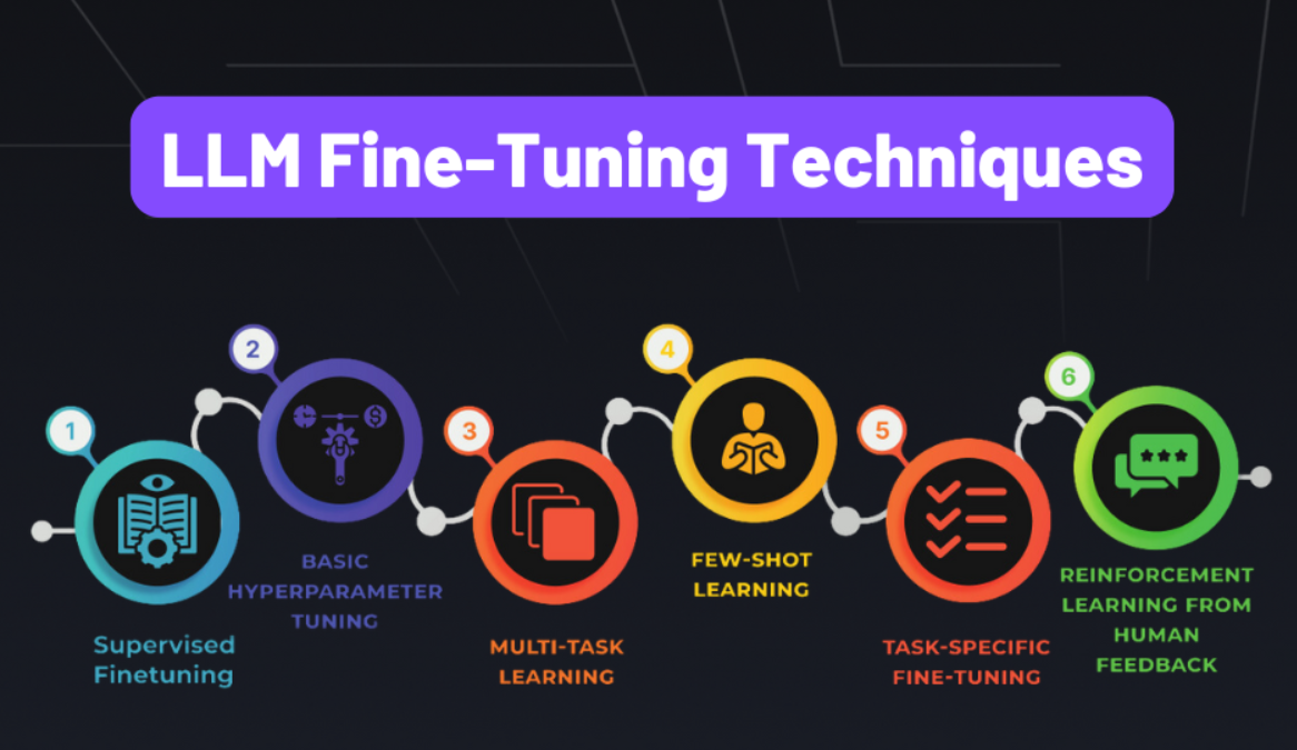
Advanced Fine-Tuning Techniques: LoRA, QLoRA, PEFT, and RLHF

Introduction

Fine-tuning large language models (LLMs) on custom data is essential for adapting them to specific domains, tasks, or organizational needs. However, full fine-tuning of billion-parameter models is prohibitively expensive in terms of compute, memory, and storage. This article provides a comprehensive deep dive into Parameter-Efficient Fine-Tuning (PEFT) techniques that achieve comparable or superior results while updating only a small fraction of model parameters.

What You’ll Learn

• LoRA & QLoRA: Memory-efficient adaptation with low-rank matrices
• PEFT Methods: Prefix tuning, prompt tuning, IA³, and adapter techniques
• Instruction Tuning: Teaching models to follow instructions effectively
• RLHF & DPO: Aligning models with human preferences
• Production Strategies: Real-world deployment patterns and optimization
• Advanced Techniques: Recent innovations from 2024-2025

Target Audience: ML Engineers, AI Researchers, and practitioners working with LLMs who need practical, production-ready fine-tuning solutions.

The Challenge: Full Fine-Tuning Limitations

Resource Requirements

Full fine-tuning requires updating all model parameters, leading to substantial computational overhead:

# Full fine-tuning a 7B parameter model
model = AutoModelForCausalLM.from_pretrained("meta-llama/Llama-2-7b-hf")

# Memory required: ~28GB (FP32) or ~14GB (FP16) just to load
# Training memory: 3-4x model size = ~56GB+ GPU RAM
# Storage: Need to save entire 7B parameters for each checkpoint

Critical Problems

Challenge	Impact	Cost Multiplier
Hardware Requirements	A100 80GB+ needed	$2-3/hour
Catastrophic Forgetting	Loss of pre-trained knowledge	Quality degradation
Storage Overhead	Multiple full checkpoints	10-50GB per version
Training Time	Days to weeks	High opportunity cost
Overfitting Risk	Especially on small datasets	Poor generalization

The PEFT Solution

Parameter-Efficient Fine-Tuning addresses these challenges by:

• ✅ Updating <1% of parameters while maintaining performance
• ✅ Reducing memory requirements by 3-10x
• ✅ Enabling multi-task serving with adapter switching
• ✅ Preserving pre-trained knowledge through selective updates

1. LoRA (Low-Rank Adaptation)

Paper: LoRA: Low-Rank Adaptation of Large Language Models (Hu et al., 2021)
Impact: 10,000+ citations, industry standard for efficient fine-tuning

Technique Overview: LoRA is a parameter-efficient fine-tuning method that freezes the original model weights and injects trainable low-rank matrices into each layer. Instead of updating billions of parameters, LoRA trains only small adapter matrices (typically <1% of total parameters), dramatically reducing memory requirements and training costs while achieving comparable performance to full fine-tuning. This makes it possible to fine-tune large models on consumer GPUs and enables efficient multi-task deployment through adapter switching.

Core Concept

Instead of updating all model weights W, LoRA adds trainable low-rank decomposition matrices B and A:

W’ = W + BA

Where:

• W: Original frozen weights (d × k dimensions)
• B: Trainable down-projection matrix (d × r dimensions)
• A: Trainable up-projection matrix (r × k dimensions)
• r: Rank (typically 4-64), much smaller than d and k
• ΔW = BA: Low-rank update

Key Insight: The intrinsic rank of task-specific weight updates is much smaller than the full weight matrix dimensionality. LoRA exploits this by constraining updates to a low-rank subspace.

Mathematical Foundation

For a pre-trained weight matrix W₀, the forward pass becomes:

h = W₀x + ΔWx = W₀x + BAx

During training:

• W₀ remains frozen (no gradients computed)
• Only A and B are updated via backpropagation
• Scaling factor α/r controls adaptation strength

The effective learning rate for LoRA weights: η_LoRA = η · (α/r)

Implementation with Best Practices

from transformers import AutoModelForCausalLM, AutoTokenizer
from peft import LoraConfig, get_peft_model, TaskType

# Load base model
model = AutoModelForCausalLM.from_pretrained(
    "meta-llama/Llama-2-7b-hf",
    torch_dtype=torch.float16,
    device_map="auto"
)

# LoRA configuration
lora_config = LoraConfig(
    task_type=TaskType.CAUSAL_LM,
    r=16,                          # Rank
    lora_alpha=32,                 # Scaling factor
    lora_dropout=0.05,             # Dropout for regularization
    target_modules=["q_proj", "v_proj"],  # Which layers to adapt
    bias="none"
)

# Wrap model with LoRA
model = get_peft_model(model, lora_config)
model.print_trainable_parameters()
# Output: trainable params: 4,194,304 || all params: 6,742,609,920 || trainable%: 0.062%

# Training
from transformers import Trainer, TrainingArguments

training_args = TrainingArguments(
    output_dir="./lora-llama2",
    per_device_train_batch_size=4,
    gradient_accumulation_steps=4,
    num_train_epochs=3,
    learning_rate=2e-4,
    fp16=True,
    logging_steps=10,
    save_strategy="epoch"
)

trainer = Trainer(
    model=model,
    args=training_args,
    train_dataset=tokenized_dataset,
)

trainer.train()

# Save LoRA weights (only ~10MB!)
model.save_pretrained("./lora-weights")

LoRA Advantages

Benefit	Description	Impact
Memory Efficiency	0.01-1% of parameters trained	10-100x reduction
Training Speed	3x faster than full fine-tuning	Cost savings
Modularity	Swap adapters without reloading base	Multi-task serving
No Inference Latency	Merge adapters with base weights	Production ready
Catastrophic Forgetting Prevention	Base model remains intact	Preserves capabilities

Advanced LoRA Techniques (2024-2025)

1. LoRA+ (Improved Optimizer)

# LoRA+ uses different learning rates for A and B matrices
from peft import LoraConfig

config = LoraConfig(
    r=16,
    lora_alpha=32,
    # Use higher LR for B matrix (empirically better)
    use_rslora=True,  # Rank-stabilized LoRA
)

2. DoRA (Weight-Decomposed LoRA)

Technique Overview: DoRA (Weight-Decomposed Low-Rank Adaptation) improves upon standard LoRA by decomposing pre-trained weights into magnitude and direction components, applying low-rank updates only to the directional component. This decomposition better captures the learning patterns observed in full fine-tuning, leading to improved performance over vanilla LoRA with the same number of trainable parameters. DoRA consistently outperforms LoRA across various tasks while maintaining similar computational efficiency.

# DoRA: Decomposes weights into magnitude and direction
config = LoraConfig(
    r=16,
    use_dora=True,  # Enable DoRA
    lora_alpha=16,
)
# Better performance than standard LoRA with same parameters

3. AdaLoRA (Adaptive Rank Allocation)

Technique Overview: AdaLoRA dynamically allocates different ranks to different weight matrices during training based on their importance, rather than using a fixed rank across all layers. It starts with higher ranks and progressively prunes less important singular values, concentrating parameters where they matter most. This adaptive approach achieves better parameter efficiency than fixed-rank LoRA, automatically discovering which layers benefit from higher-rank adaptation and which can use minimal parameters.

from peft import AdaLoraConfig

# Dynamically adjusts rank across layers
config = AdaLoraConfig(
    r=8,  # Average rank
    target_r=4,  # Target rank after pruning
    init_r=12,  # Initial rank
    tinit=200,  # Warmup steps
    tfinal=1000,  # Total steps
    deltaT=10,  # Update interval
)

LoRA Best Practices

# Target modules selection
# For Llama/GPT models:
target_modules = ["q_proj", "k_proj", "v_proj", "o_proj", "gate_proj", "up_proj", "down_proj"]

# For BERT models:
target_modules = ["query", "key", "value"]

# Rank selection (empirical):
# - r=4-8: Simple tasks (classification, small datasets)
# - r=16-32: Complex tasks (dialogue, summarization)
# - r=64+: Very specialized domains (legal, medical)

# Alpha scaling:
# lora_alpha = 2 * r is a good default

Multi-Adapter Inference

from peft import PeftModel

# Load base model once
base_model = AutoModelForCausalLM.from_pretrained("meta-llama/Llama-2-7b-hf")

# Load different adapters for different tasks
model_task1 = PeftModel.from_pretrained(base_model, "./lora-customer-support")
model_task2 = PeftModel.from_pretrained(base_model, "./lora-code-generation")

# Switch adapters dynamically
model_task1.set_adapter("customer-support")
response = model_task1.generate(...)

2. QLoRA (Quantized LoRA)

Paper: QLoRA: Efficient Finetuning of Quantized LLMs (Dettmers et al., 2023)
Breakthrough: Fine-tune 65B models on a single 48GB GPU, 33B on 24GB GPU

Technique Overview: QLoRA pushes memory efficiency to the extreme by combining LoRA with 4-bit quantization of the base model. This groundbreaking approach uses NormalFloat4 quantization, double quantization of constants, and paged optimizers to reduce memory consumption by 5-6x compared to standard LoRA. QLoRA democratizes fine-tuning of massive models (70B+ parameters) on consumer hardware without significant quality degradation, making state-of-the-art model adaptation accessible to researchers and practitioners with limited resources.

Innovation

QLoRA combines LoRA with 4-bit quantization to achieve unprecedented memory efficiency without sacrificing performance. Enables fine-tuning massive models on consumer hardware.

Key Technical Components

1. 4-bit NormalFloat (NF4)

Optimal quantization for normally distributed weights (common in neural networks):

NF4 = {qᵢ} where qᵢ partitions N(0,1) into equal-area buckets

2. Double Quantization

Quantizes the quantization constants themselves:

Memory Savings Calculation:
- Standard 4-bit: 0.5 bytes per parameter + 32-bit constants
- Double quantization: 0.5 bytes + 8-bit constants
- Savings: ~0.37 bytes per parameter (26% reduction in quantization overhead)

3. Paged Optimizers

Uses unified memory (CPU + GPU) via NVIDIA’s Unified Memory to handle optimizer states:

# Automatically page to CPU when GPU is full
optimizer = bnb.optim.PagedAdamW32bit(model.parameters())

Implementation

from transformers import AutoModelForCausalLM, BitsAndBytesConfig
from peft import prepare_model_for_kbit_training, LoraConfig, get_peft_model

# 4-bit quantization config
bnb_config = BitsAndBytesConfig(
    load_in_4bit=True,
    bnb_4bit_quant_type="nf4",           # NormalFloat4
    bnb_4bit_compute_dtype=torch.bfloat16,  # Compute in BF16
    bnb_4bit_use_double_quant=True,      # Double quantization
)

# Load model in 4-bit
model = AutoModelForCausalLM.from_pretrained(
    "meta-llama/Llama-2-70b-hf",  # 70B model!
    quantization_config=bnb_config,
    device_map="auto"
)

# Prepare for k-bit training
model = prepare_model_for_kbit_training(model)

# Add LoRA adapters
lora_config = LoraConfig(
    r=64,
    lora_alpha=128,
    target_modules=["q_proj", "k_proj", "v_proj", "o_proj"],
    lora_dropout=0.05,
    bias="none",
    task_type="CAUSAL_LM"
)

model = get_peft_model(model, lora_config)

# Train (fits in 24GB GPU!)
trainer = Trainer(
    model=model,
    train_dataset=dataset,
    args=TrainingArguments(
        per_device_train_batch_size=1,
        gradient_accumulation_steps=16,
        learning_rate=2e-4,
        bf16=True,  # Use bfloat16
        optim="paged_adamw_8bit",  # 8-bit optimizer
    )
)

trainer.train()

QLoRA Performance

Model	Params	Full FT Memory	QLoRA Memory	Reduction	Accuracy Loss
Llama-2-7B	7B	28GB	6GB	4.7x	<0.5%
Llama-2-13B	13B	52GB	10GB	5.2x	<0.7%
Llama-2-70B	70B	280GB	48GB	5.8x	<1.5%
Falcon-40B	40B	160GB	28GB	5.7x	<1.2%

Key Insight: QLoRA achieves 99%+ of full fine-tuning quality at 1/5th the memory cost.

Production Considerations

# Inference optimization: Merge and dequantize for deployment
from peft import PeftModel

# Load quantized model + adapter
base_model = AutoModelForCausalLM.from_pretrained(
    "model_id",
    quantization_config=bnb_config
)
model = PeftModel.from_pretrained(base_model, "qlora_adapter")

# Merge adapter
merged = model.merge_and_unload()

# Dequantize to FP16 for faster inference
merged_fp16 = merged.to(torch.float16)
merged_fp16.save_pretrained("production_model")

3. Other PEFT Methods

a. Prefix Tuning

Technique Overview: Prefix Tuning prepends learnable continuous vectors (soft prompts) to the input of each transformer layer, acting as virtual tokens that guide the model’s behavior. Unlike prompt engineering with discrete tokens, these prefix embeddings are optimized during training to steer the frozen model toward task-specific outputs. This method is extremely parameter-efficient (typically 0.01-0.1% trainable parameters) and works well for multi-task scenarios where different prefixes can be applied for different tasks.

Add trainable “virtual tokens” to the input.

from peft import PrefixTuningConfig, get_peft_model

config = PrefixTuningConfig(
    task_type=TaskType.CAUSAL_LM,
    num_virtual_tokens=20,  # Number of prefix tokens
    encoder_hidden_size=4096
)

model = get_peft_model(base_model, config)

b. Prompt Tuning

Technique Overview: Prompt Tuning is a simplified version of prefix tuning that only adds learnable embeddings to the input layer (not every transformer layer). By training a small set of continuous prompt tokens while keeping the entire model frozen, this approach achieves remarkable efficiency with as few as 0.001-0.01% trainable parameters. It’s particularly effective for few-shot learning and adapting models to simple classification or extraction tasks with minimal computational overhead.

Similar to prefix tuning but simpler (only input embeddings).

from peft import PromptTuningConfig

config = PromptTuningConfig(
    task_type=TaskType.CAUSAL_LM,
    num_virtual_tokens=8,
    prompt_tuning_init="TEXT",  # Initialize from text
    prompt_tuning_init_text="Classify if the text is positive or negative:"
)

c. IA³ (Infused Adapter by Inhibiting and Amplifying Inner Activations)

Technique Overview: IA³ introduces trainable scaling vectors that multiplicatively modify key, value, and feedforward activations within the transformer. Instead of adding parameters like LoRA or adapters, IA³ learns to amplify or inhibit existing activations through element-wise multiplication. This results in one of the most parameter-efficient methods available (often <0.01% trainable parameters) while maintaining high performance, making it ideal for scenarios requiring minimal storage and ultra-fast adapter switching.

Learns scaling vectors for attention and feedforward activations.

from peft import IA3Config

config = IA3Config(
    task_type=TaskType.CAUSAL_LM,
    target_modules=["k_proj", "v_proj", "down_proj"],
    feedforward_modules=["down_proj"]
)

PEFT Methods Comparison

Method	Trainable %	Memory	Inference Speed	Training Stability	Best Use Case
Full Fine-tuning	100%	Highest	Fast	High	Unlimited resources, small models
LoRA	0.1-1%	Low	Fast	High	General purpose, production
QLoRA	0.1-1%	Lowest	Fast	High	Large models, limited GPU
Prefix Tuning	0.01-0.1%	Very Low	Medium	Medium	Multi-task, few-shot
Prompt Tuning	0.001-0.01%	Very Low	Medium	Low	Simple tasks, embeddings
IA³	0.01%	Very Low	Fast	High	Extremely lightweight
Adapter Layers	0.5-5%	Medium	Slow	High	Legacy compatibility

Emerging PEFT Methods (2024-2025)

a. VeRA (Vector-based Random Matrix Adaptation)

Technique Overview: VeRA dramatically reduces trainable parameters by using shared frozen random matrices across all layers, training only small scaling vectors per layer. Instead of learning separate A and B matrices like LoRA, VeRA leverages a single pair of frozen random projections shared across the model, requiring only learnable scaling vectors (b and d). This innovation enables using much higher ranks (256+) while training 10x fewer parameters than LoRA, achieving comparable performance with minimal memory overhead.

from peft import VeraConfig

# Uses shared random matrices, only trains scaling vectors
config = VeraConfig(
    r=256,  # Can use much higher rank
    target_modules=["q_proj", "v_proj"],
    vera_dropout=0.0,
)
# 10x fewer parameters than LoRA with similar performance

b. (IA)³ with Task Vectors

# Combine multiple task adaptations
base_model = load_model("base")
task1_model = load_model("task1_ia3")
task2_model = load_model("task2_ia3")

# Arithmetic on task vectors
combined_weights = 0.5 * task1_weights + 0.5 * task2_weights

4. Instruction Tuning

Goal: Transform base models into instruction-following assistants like ChatGPT.

Technique Overview: Instruction Tuning fine-tunes language models on datasets of (instruction, input, output) triplets to teach them how to follow natural language commands and perform diverse tasks. While pre-trained models excel at text completion, they don’t naturally understand task specifications in plain language. This supervised fine-tuning phase transforms raw language models into versatile assistants that can interpret instructions, follow multi-step directions, and generate helpful responses across various domains—forming the foundation for chat-based AI systems.

The Instruction Tuning Paradigm

Base models predict next tokens but don’t naturally follow instructions. Instruction tuning bridges this gap through supervised fine-tuning on instruction-response pairs.

Instruction Dataset Format

# Standard instruction format
instruction_data = [
    {
        "instruction": "Summarize the following article in 2 sentences.",
        "input": "Article text here...",
        "output": "Summary of the article."
    },
    {
        "instruction": "Translate the following to French.",
        "input": "Hello, how are you?",
        "output": "Bonjour, comment allez-vous?"
    }
]

# Alpaca format (widely adopted)
alpaca_prompt = """Below is an instruction that describes a task, paired with an input that provides further context. Write a response that appropriately completes the request.

### Instruction:
{instruction}

### Input:
{input}

### Response:
{output}"""

# ChatML format (OpenAI-style)
chatml_format = """<|im_start|>system
You are a helpful assistant.<|im_end|>
<|im_start|>user
{instruction}<|im_end|>
<|im_start|>assistant
{output}<|im_end|>"""

# Llama-2 Chat format
llama2_format = """<s>[INST] <<SYS>>
{system_prompt}
<</SYS>>

{instruction} [/INST] {output} </s>"""

Training on Instructions

from datasets import load_dataset

# Load instruction dataset
dataset = load_dataset("tatsu-lab/alpaca")  # 52K instructions

# Format for training
def format_instruction(example):
    prompt = alpaca_prompt.format(
        instruction=example["instruction"],
        input=example["input"],
        output=""
    )
    return {"text": prompt, "label": example["output"]}

formatted_dataset = dataset.map(format_instruction)

# Fine-tune with LoRA
# ... (same as previous LoRA code)

Popular Instruction Datasets

Dataset	Size	Source	Focus	License
Alpaca	52K	Stanford	General instructions	CC BY-NC 4.0
Dolly-15k	15K	Databricks	Human-generated	CC BY-SA 3.0
FLAN	1.8M	Google	Multi-task instructions	Apache 2.0
OpenAssistant	161K	LAION	Conversational	Apache 2.0
ShareGPT	90K	Community	ChatGPT conversations	Various
Orca	5M	Microsoft	GPT-4 explanations	Research only
UltraChat	1.4M	Tsinghua	Multi-turn dialogues	MIT
WizardLM	250K	Microsoft	Complex instructions	Research only

Advanced Instruction Tuning Strategies

1. Multi-Task Instruction Tuning

# Mix different task types for better generalization
from datasets import concatenate_datasets

qa_dataset = load_dataset("squad_v2")
summarization = load_dataset("cnn_dailymail")
translation = load_dataset("wmt14")

mixed_dataset = concatenate_datasets([
    format_as_instructions(qa_dataset),
    format_as_instructions(summarization),
    format_as_instructions(translation),
])

2. Self-Instruct Pipeline

Generate synthetic instructions using the model itself:

# Bootstrap from seed instructions
seed_instructions = ["Explain...", "Summarize...", "Translate..."]

# Generate new instructions
def self_instruct(seed, model, num_generate=1000):
    generated = []
    for _ in range(num_generate):
        prompt = f"Generate a diverse instruction:\n{random.choice(seed)}"
        new_instruction = model.generate(prompt)
        generated.append(new_instruction)
    return generated

# Filter and curate
high_quality = filter_by_quality(generated_instructions)

5. RLHF (Reinforcement Learning from Human Feedback)

Used by: ChatGPT, Claude, Gemini, Llama 2, GPT-4

Core Idea: Optimize models to maximize human preferences rather than just likelihood.

Technique Overview: RLHF aligns language models with human values and preferences through a three-stage process: supervised fine-tuning on demonstrations, training a reward model from human preference comparisons, and reinforcement learning (typically PPO) to optimize the policy against the reward model. This technique addresses the limitation that maximum likelihood training doesn’t capture nuanced human preferences like helpfulness, harmlessness, and honesty. RLHF is the secret sauce behind models like ChatGPT, enabling them to refuse harmful requests, admit uncertainty, and provide responses that humans find genuinely useful rather than just statistically likely.

Three-Stage RLHF Process

Stage 1: Supervised Fine-Tuning (SFT)

Train on high-quality human demonstrations:

# Train on high-quality demonstrations
sft_dataset = load_dataset("openassistant-guanaco")

# Standard supervised fine-tuning
trainer = Trainer(model=model, train_dataset=sft_dataset)
trainer.train()

# Critical: SFT provides the initial policy for RL

SFT Best Practices:

• Use 10K-100K high-quality examples
• Focus on desired behavior patterns
• Include diverse instruction types
• Train for 1-3 epochs to avoid overfitting

Stage 2: Reward Model Training

Train a model to score responses based on human preferences:

from transformers import AutoModelForSequenceClassification

# Dataset: (prompt, response_chosen, response_rejected)
preference_data = [
    {
        "prompt": "Explain quantum computing",
        "chosen": "Quantum computing uses quantum bits...",  # Human preferred
        "rejected": "It's like magic computers..."  # Human rejected
    }
]

# Train reward model
reward_model = AutoModelForSequenceClassification.from_pretrained(
    "meta-llama/Llama-2-7b-hf",
    num_labels=1  # Scalar reward
)

# Bradley-Terry loss
def reward_loss(chosen_reward, rejected_reward):
    return -torch.log(torch.sigmoid(chosen_reward - rejected_reward))

# Train to predict: reward(chosen) > reward(rejected)

Reward Model Architecture:

• Same base as language model
• Replace LM head with regression head
• Output: scalar reward score
• Training: 50K-300K preference pairs

Stage 3: PPO (Proximal Policy Optimization)

from trl import PPOTrainer, PPOConfig, AutoModelForCausalLMWithValueHead

# Load SFT model
model = AutoModelForCausalLMWithValueHead.from_pretrained("./sft-model")

# PPO configuration
ppo_config = PPOConfig(
    batch_size=16,
    learning_rate=1.41e-5,
    log_with="wandb",
)

# PPO Trainer
ppo_trainer = PPOTrainer(
    config=ppo_config,
    model=model,
    ref_model=reference_model,  # Original SFT model
    tokenizer=tokenizer,
)

# Training loop
for batch in dataset:
    # Generate responses
    response_tensors = ppo_trainer.generate(batch["query"])
    
    # Get rewards from reward model
    rewards = [reward_model(r).item() for r in response_tensors]
    
    # PPO update
    stats = ppo_trainer.step(batch["query"], response_tensors, rewards)

Simplified RLHF with DPO (Direct Preference Optimization)

Paper: Direct Preference Optimization (Rafailov et al., 2023)
Breakthrough: Eliminates reward model and RL complexity

Technique Overview: DPO revolutionizes preference learning by bypassing the complex reward modeling and reinforcement learning stages of traditional RLHF. It directly optimizes the language model on preference pairs using a classification-style loss function, treating the alignment problem as supervised learning rather than RL. By mathematically reparameterizing the RL objective, DPO achieves comparable or better results than PPO-based RLHF with dramatically simpler implementation, fewer hyperparameters, greater training stability, and lower computational costs—making preference alignment accessible to practitioners without RL expertise.

Why DPO is Revolutionary

Aspect	RLHF (PPO)	DPO
Training Stages	3 (SFT → RM → PPO)	2 (SFT → DPO)
Reward Model	Required	Not needed
Hyperparameters	15-20 critical params	3-5 simple params
Training Stability	Unstable (RL)	Stable (supervised)
Implementation	Complex	Simple
Compute Cost	High	Medium

DPO Mathematical Foundation

DPO reparameterizes the RL objective as a classification problem. The loss function compares the probability ratios of preferred vs rejected responses under the current policy versus the reference policy.

Where:

• y_w: Preferred (winning) response
• y_l: Rejected (losing) response
• β: Temperature parameter (controls KL penalty)
• π_ref: Reference policy (SFT model)

from trl import DPOTrainer, DPOConfig

# Load SFT model
model = AutoModelForCausalLM.from_pretrained("./sft-model")
ref_model = AutoModelForCausalLM.from_pretrained("./sft-model")  # Reference

# Preference dataset
dataset = load_dataset("Anthropic/hh-rlhf")

# DPO configuration
dpo_config = DPOConfig(
    beta=0.1,  # KL divergence penalty (0.1-0.5)
    learning_rate=5e-7,
    max_length=1024,
    max_prompt_length=512,
)

# DPO training (much simpler than PPO!)
trainer = DPOTrainer(
    model=model,
    ref_model=ref_model,
    args=dpo_config,
    train_dataset=dataset,
    tokenizer=tokenizer,
)

trainer.train()

Advanced Preference Learning (2024-2025)

1. IPO (Identity Preference Optimization)

Technique Overview: IPO simplifies preference optimization by using an identity mapping instead of the log probability ratios used in DPO. This modification results in more stable training gradients and eliminates the need to maintain a reference model during inference. IPO achieves similar alignment quality to DPO while being more robust to hyperparameter choices and requiring less computational overhead, making it an attractive alternative for practitioners seeking simpler, more stable preference learning.

# More stable than DPO, doesn't require reference model at inference
from trl import IPOTrainer

trainer = IPOTrainer(
    model=model,
    train_dataset=dataset,
    beta=0.1,  # Simpler than DPO
)

2. KTO (Kahneman-Tversky Optimization)

Technique Overview: KTO revolutionizes preference learning by eliminating the need for pairwise comparisons, working instead with simple binary feedback (good/bad, thumbs up/down). Inspired by Kahneman-Tversky prospect theory, KTO models human preferences using separate utility functions for gains and losses. This approach dramatically reduces data collection costs since annotators only need to judge individual responses rather than compare pairs, while achieving comparable or better alignment than DPO with significantly less human effort.

# Works with simple thumbs up/down, no pairwise comparisons needed
from trl import KTOTrainer

# Dataset format: (prompt, response, label)
# label: True (good) or False (bad)
kto_dataset = [
    {"prompt": "...", "response": "...", "label": True},
]

trainer = KTOTrainer(
    model=model,
    train_dataset=kto_dataset,
    desirable_weight=1.0,
    undesirable_weight=1.0,
)

3. ORPO (Odds Ratio Preference Optimization)

Technique Overview: ORPO is a groundbreaking single-stage method that combines supervised fine-tuning and preference alignment into one unified training process. By using odds ratios to contrast preferred and rejected responses, ORPO eliminates the need for a separate SFT stage, reducing training time and computational costs by 50%. This monolithic approach maintains competitive performance with multi-stage methods while simplifying the training pipeline and reducing the risk of distribution shift between training stages.

# Combines SFT and preference learning in one stage
from trl import ORPOTrainer

trainer = ORPOTrainer(
    model=model,
    train_dataset=preference_dataset,
    # No need for separate SFT stage!
)

DPO Advantages:

• ✅ No reward model needed (50% less training)
• ✅ Simpler than PPO (5x fewer hyperparameters)
• ✅ More stable training (supervised learning)
• ✅ Comparable or better results to RLHF
• ✅ Lower computational cost

6. Practical Fine-Tuning Pipeline

Complete Example: Domain-Specific Chatbot

# Step 1: Prepare dataset
from datasets import Dataset

data = {
    "instruction": [...],
    "input": [...],
    "output": [...]
}
dataset = Dataset.from_dict(data)

# Step 2: Load model with QLoRA
model = AutoModelForCausalLM.from_pretrained(
    "meta-llama/Llama-2-7b-chat-hf",
    quantization_config=BitsAndBytesConfig(load_in_4bit=True),
    device_map="auto"
)

# Step 3: Add LoRA adapters
model = prepare_model_for_kbit_training(model)
lora_config = LoraConfig(r=16, lora_alpha=32, target_modules=["q_proj", "v_proj"])
model = get_peft_model(model, lora_config)

# Step 4: Train
trainer = Trainer(
    model=model,
    train_dataset=dataset,
    args=TrainingArguments(
        per_device_train_batch_size=4,
        gradient_accumulation_steps=4,
        num_train_epochs=3,
        learning_rate=2e-4,
        fp16=True,
        logging_steps=10,
        output_dir="./output"
    )
)

trainer.train()

# Step 5: Save and merge
model.save_pretrained("./lora-adapter")

# Optional: Merge for faster inference
merged_model = model.merge_and_unload()
merged_model.save_pretrained("./merged-model")

7. Best Practices & Tips

When to Use What

Decision Tree:

Start
├─ Budget limited? 
│  ├─ Yes → QLoRA (4-bit)
│  └─ No → Continue
├─ Model size?
│  ├─ < 7B → LoRA or Full FT
│  ├─ 7B-30B → LoRA
│  └─ > 30B → QLoRA
├─ Multiple tasks?
│  ├─ Yes → LoRA (adapter switching)
│  └─ No → Continue
├─ Need alignment?
│  ├─ Yes → SFT + DPO
│  └─ No → Instruction tuning
└─ Production latency critical?
   ├─ Yes → Merge adapters
   └─ No → Load adapters dynamically

Comprehensive Hyperparameter Guide

# Learning Rates (empirically validated)
learning_rates = {
    "full_ft": 1e-5 to 5e-5,
    "lora": 1e-4 to 3e-4,
    "qlora": 2e-4 to 5e-4,
    "dpo": 5e-7 to 5e-6,  # Much lower!
}

# LoRA Rank Selection
rank_guide = {
    "simple_classification": 4,
    "qa_extraction": 8,
    "general_chat": 16,
    "complex_reasoning": 32,
    "domain_expert": 64,
    "code_generation": 64,
}

# Alpha scaling (rule of thumb)
# lora_alpha = 2 * r  (standard)
# lora_alpha = r      (conservative, less forgetting)
# lora_alpha = 4 * r  (aggressive adaptation)

# Batch Size Optimization
def calculate_batch_size(gpu_memory_gb, model_size_b):
    # Rough heuristic
    effective_batch = (gpu_memory_gb * 0.8) / (model_size_b * 2)
    per_device_batch = max(1, int(effective_batch / 4))
    grad_accum_steps = max(1, 16 // per_device_batch)
    return per_device_batch, grad_accum_steps

# Example: 24GB GPU, 7B model
batch_size, grad_accum = calculate_batch_size(24, 7)
# Returns: batch_size=2, grad_accum=8
# Effective batch size = 2 * 8 = 16

Training Duration & Convergence

# Epochs by dataset size
epoch_guide = {
    "tiny": (100, 1000, 10, 20),      # size range, min epochs, max epochs
    "small": (1000, 10000, 5, 10),
    "medium": (10000, 100000, 3, 5),
    "large": (100000, 1000000, 1, 3),
    "xlarge": (1000000, float('inf'), 1, 2),
}

# Early stopping configuration
early_stopping_config = {
    "patience": 3,  # Epochs without improvement
    "threshold": 0.01,  # Minimum improvement
    "metric": "eval_loss",
}

# Learning rate scheduling
from transformers import get_scheduler

scheduler = get_scheduler(
    "cosine",  # or "linear", "polynomial"
    optimizer=optimizer,
    num_warmup_steps=100,  # 3-10% of total steps
    num_training_steps=total_steps,
)

Preventing Overfitting

# 1. Dropout regularization
lora_config = LoraConfig(
    lora_dropout=0.05,  # 0.05-0.1 recommended
)

# 2. Early stopping
from transformers import EarlyStoppingCallback

trainer = Trainer(
    callbacks=[EarlyStoppingCallback(
        early_stopping_patience=3,
        early_stopping_threshold=0.001,
    )]
)

# 3. Weight decay (L2 regularization)
training_args = TrainingArguments(
    weight_decay=0.01,  # 0.01-0.1
    warmup_ratio=0.03,  # 3% warmup
    max_grad_norm=1.0,  # Gradient clipping
)

# 4. Data augmentation
from datasets import concatenate_datasets

def augment_instruction_data(example):
    # Paraphrase instructions
    variations = [
        example["instruction"],
        rephrase(example["instruction"]),
        simplify(example["instruction"]),
    ]
    return variations

# 5. Monitor training curves
import wandb

wandb.init(project="fine-tuning")

# Log every N steps
training_args = TrainingArguments(
    logging_steps=10,
    eval_steps=100,
    save_steps=500,
    load_best_model_at_end=True,
    metric_for_best_model="eval_loss",
)

8. Evaluation & Benchmarking

Quantitative Evaluation

from lm_eval import evaluator

# Standard benchmarks
benchmarks = {
    "mmlu": "Massive Multitask Language Understanding",
    "hellaswag": "Commonsense reasoning",
    "arc_challenge": "Science questions",
    "truthfulqa": "Truthfulness",
    "gsm8k": "Math reasoning",
}

# Run evaluation
results = evaluator.simple_evaluate(
    model="hf",
    model_args="pretrained=./fine-tuned-model",
    tasks=["mmlu", "hellaswag", "arc_challenge"],
    num_fewshot=0,
    batch_size=8,
)

print(f"MMLU: {results['results']['mmlu']['acc']:.2%}")
print(f"HellaSwag: {results['results']['hellaswag']['acc_norm']:.2%}")

Domain-Specific Evaluation

# Custom evaluation suite
def evaluate_domain_model(model, tokenizer, test_set):
    metrics = {
        "accuracy": [],
        "f1_score": [],
        "rouge_l": [],
        "bleu": [],
    }
    
    for example in test_set:
        prediction = model.generate(
            example["input"],
            max_new_tokens=256,
            temperature=0.7,
        )
        
        # Task-specific metrics
        if example["task"] == "classification":
            metrics["accuracy"].append(
                accuracy_score(example["label"], prediction)
            )
        elif example["task"] == "generation":
            metrics["rouge_l"].append(
                rouge_score(example["reference"], prediction)
            )
    
    return {k: np.mean(v) for k, v in metrics.items()}

Human Evaluation Framework

# A/B testing framework
def human_evaluation(model_a, model_b, prompts):
    results = {"model_a_wins": 0, "model_b_wins": 0, "ties": 0}
    
    for prompt in prompts:
        response_a = model_a.generate(prompt)
        response_b = model_b.generate(prompt)
        
        # Present to human evaluators (randomized)
        preference = get_human_preference(response_a, response_b)
        
        if preference == "a":
            results["model_a_wins"] += 1
        elif preference == "b":
            results["model_b_wins"] += 1
        else:
            results["ties"] += 1
    
    return results

# LLM-as-judge (automated evaluation)
def llm_judge_evaluation(judge_model, model_output, reference):
    prompt = f"""Rate the following response on a scale of 1-10:
    
Reference: {reference}
Response: {model_output}

Criteria:
- Accuracy (1-3 points)
- Completeness (1-3 points)
- Clarity (1-2 points)
- Helpfulness (1-2 points)

Score:"""
    
    score = judge_model.generate(prompt)
    return int(score)

Performance Comparison Table

Model	MMLU	HellaSwag	TruthfulQA	GSM8K	Training Time	Cost
Base Llama-2-7B	45.3%	77.2%	38.8%	14.6%	-	-
Full Fine-tuned	52.1%	81.5%	45.2%	28.3%	48h	$384
LoRA (r=16)	51.8%	81.2%	44.9%	27.8%	16h	$128
QLoRA (r=16)	51.5%	80.9%	44.5%	27.2%	18h	$72
+ DPO	53.2%	82.1%	56.7%	29.1%	+8h	+$32

9. Troubleshooting Guide

Common Issues & Solutions

Issue 1: Out of Memory (OOM)

# Solution strategies (in order of preference)

# 1. Reduce batch size
per_device_batch_size = 1
gradient_accumulation_steps = 16  # Keep effective batch size

# 2. Enable gradient checkpointing
model.gradient_checkpointing_enable()

# 3. Use QLoRA instead of LoRA
quantization_config = BitsAndBytesConfig(load_in_4bit=True)

# 4. Reduce sequence length
max_length = 512  # Instead of 2048

# 5. Use Flash Attention 2
model = AutoModelForCausalLM.from_pretrained(
    model_id,
    attn_implementation="flash_attention_2",
    torch_dtype=torch.float16,
)

# 6. Optimize optimizer memory
from bitsandbytes.optim import AdamW8bit
optimizer = AdamW8bit(model.parameters())

Issue 2: Training Instability / Loss Spikes

# Diagnosis
import matplotlib.pyplot as plt

# Plot training loss
plt.plot(trainer.state.log_history["loss"])
plt.show()

# Solutions:

# 1. Lower learning rate
learning_rate = 5e-5  # Reduce by 2-5x

# 2. Add warmup
warmup_steps = int(0.1 * total_steps)

# 3. Gradient clipping
max_grad_norm = 0.3  # More aggressive

# 4. Use bf16 instead of fp16 (better numerical stability)
training_args = TrainingArguments(
    bf16=True,  # Instead of fp16=True
)

# 5. Check for bad data
def validate_dataset(dataset):
    for i, example in enumerate(dataset):
        if len(example["input_ids"]) > max_length:
            print(f"Example {i} too long: {len(example['input_ids'])}")
        if example["input_ids"].max() >= vocab_size:
            print(f"Example {i} has invalid token")

Issue 3: Model Not Learning (Loss Plateau)

# Diagnosis: loss not decreasing

# Solutions:

# 1. Increase learning rate
learning_rate = 3e-4  # Up from 1e-4

# 2. Increase LoRA rank
r = 32  # Up from 8

# 3. Target more modules
target_modules = [
    "q_proj", "k_proj", "v_proj", "o_proj",
    "gate_proj", "up_proj", "down_proj",  # Add FFN layers
]

# 4. Check if adapter is actually being trained
model.print_trainable_parameters()
# Should show >0 trainable params

# 5. Verify data quality
# Check if labels are correct
# Ensure sufficient data diversity

Issue 4: Catastrophic Forgetting

# Model loses general capabilities after fine-tuning

# Prevention strategies:

# 1. Mix in general data (10-20%)
combined_dataset = concatenate_datasets([
    specialist_data.select(range(8000)),  # 80%
    general_data.select(range(2000)),     # 20%
])

# 2. Use lower rank
lora_config = LoraConfig(r=8)  # Instead of r=64

# 3. Reduce training epochs
num_train_epochs = 1  # Instead of 3

# 4. Add KL penalty (experimental)
def kl_penalty_loss(outputs, reference_outputs, beta=0.1):
    kl_div = F.kl_div(
        F.log_softmax(outputs.logits, dim=-1),
        F.softmax(reference_outputs.logits, dim=-1),
        reduction="batchmean",
    )
    return outputs.loss + beta * kl_div

Issue 5: Slow Inference After Fine-Tuning

# Adapter loading adds latency

# Solution: Merge adapters into base model
from peft import PeftModel

base_model = AutoModelForCausalLM.from_pretrained("base_model")
peft_model = PeftModel.from_pretrained(base_model, "lora_adapter")

# Merge and save
merged_model = peft_model.merge_and_unload()
merged_model.save_pretrained("merged_model")

# Now inference is as fast as base model

8. Tools & Libraries

Essential Stack

# Core fine-tuning libraries
pip install transformers>=4.35.0      # HuggingFace transformers
pip install peft>=0.7.0               # Parameter-Efficient Fine-Tuning
pip install bitsandbytes>=0.41.0      # Quantization
pip install accelerate>=0.25.0        # Multi-GPU & optimization

# RLHF/DPO libraries
pip install trl>=0.7.0                # Transformer Reinforcement Learning
pip install datasets>=2.15.0          # Dataset loading

# Evaluation
pip install lm-eval>=0.4.0            # LM Evaluation Harness
pip install rouge-score sacrebleu     # Text generation metrics

# Experiment tracking
pip install wandb tensorboard         # Logging & visualization

# Optimization (optional)
pip install flash-attn>=2.3.0         # Flash Attention (requires CUDA)
pip install deepspeed>=0.12.0         # Distributed training

Framework Comparison

Framework	Strengths	Limitations	Best For
HuggingFace PEFT	Easy, well-documented	Limited to HF models	General purpose
Axolotl	Configuration-based, turnkey	Less flexible	Quick experiments
LLaMA-Factory	GUI, many models	Chinese-focused docs	Beginners
Ludwig	Low-code	Less control	Rapid prototyping
FastChat	RLHF support	Complex setup	Production RLHF
TRL	Modern RLHF/DPO	Cutting edge (less stable)	Research

Production Deployment Tools

# Model serving
pip install vllm                      # Fast inference server
pip install text-generation-inference # HuggingFace TGI
pip install ray[serve]                # Scalable serving

# Model optimization
pip install optimum                   # ONNX, quantization
pip install auto-gptq                 # GPTQ quantization

10. Production Deployment Strategies

Multi-Adapter Architecture

# Serve multiple specialized models efficiently
from fastapi import FastAPI
from peft import PeftModel

app = FastAPI()

# Load base model once
base_model = AutoModelForCausalLM.from_pretrained(
    "llama-2-7b",
    torch_dtype=torch.float16,
    device_map="auto",
)

# Adapter registry
adapters = {
    "customer_support": "./adapters/support",
    "code_generation": "./adapters/code",
    "creative_writing": "./adapters/creative",
    "data_analysis": "./adapters/analysis",
}

# Cache for loaded adapters
adapter_cache = {}

@app.post("/generate")
async def generate(prompt: str, task: str):
    # Load adapter if not cached
    if task not in adapter_cache:
        adapter_cache[task] = PeftModel.from_pretrained(
            base_model, 
            adapters[task]
        )
    
    model = adapter_cache[task]
    response = model.generate(prompt)
    return {"response": response}

# Memory efficient: ~7GB base + ~50MB per adapter

Quantization for Production

# Option 1: GPTQ (best quality-size tradeoff)
from auto_gptq import AutoGPTQForCausalLM

model = AutoGPTQForCausalLM.from_quantized(
    "model_id",
    device="cuda:0",
    use_safetensors=True,
    use_triton=True,  # Faster inference
)

# Option 2: AWQ (fastest inference)
from awq import AutoAWQForCausalLM

model = AutoAWQForCausalLM.from_quantized(
    "model_id",
    fuse_layers=True,  # Kernel fusion
)

# Option 3: GGUF (CPU inference)
# Use llama.cpp for deployment
# Convert: python convert.py model.bin --outtype q4_k_m

# Performance comparison (7B model):
# FP16: 14GB, 30 tokens/s
# GPTQ 4-bit: 4GB, 25 tokens/s  
# AWQ 4-bit: 4GB, 35 tokens/s
# GGUF Q4_K_M: CPU, 15 tokens/s

Horizontal Scaling with vLLM

# High-throughput serving
from vllm import LLM, SamplingParams

# Initialize with optimizations
llm = LLM(
    model="./fine-tuned-model",
    tensor_parallel_size=2,     # Multi-GPU
    gpu_memory_utilization=0.9,
    max_model_len=4096,
    enable_prefix_caching=True, # Cache common prefixes
)

# Batch inference
prompts = [...]  # 100+ prompts
sampling_params = SamplingParams(
    temperature=0.7,
    top_p=0.95,
    max_tokens=256,
)

# Processes all prompts efficiently
outputs = llm.generate(prompts, sampling_params)

# 5-10x higher throughput than naive batching

Monitoring & Observability

# Production monitoring setup
import prometheus_client
from opentelemetry import trace

# Metrics
inference_latency = prometheus_client.Histogram(
    'model_inference_latency_seconds',
    'Time spent in model inference',
)

token_throughput = prometheus_client.Counter(
    'tokens_generated_total',
    'Total tokens generated',
)

@inference_latency.time()
def generate_with_monitoring(prompt):
    start_time = time.time()
    
    with trace.get_tracer(__name__).start_as_current_span("inference"):
        output = model.generate(prompt)
        
    # Log metrics
    token_count = len(tokenizer.encode(output))
    token_throughput.inc(token_count)
    
    # Alert on anomalies
    latency = time.time() - start_time
    if latency > 5.0:  # 5 second threshold
        logger.warning(f"Slow inference: {latency:.2f}s")
    
    return output

11. Advanced Research Directions

1. Mixture of LoRA Experts (MoLE)

Technique Overview: MoLE extends the Mixture of Experts (MoE) paradigm to parameter-efficient fine-tuning by combining multiple specialized LoRA adapters with a learned gating mechanism. Each LoRA expert specializes in different aspects or domains, and the gating network dynamically routes inputs to the most appropriate expert(s) based on the input context. This architecture enables a single model to handle diverse tasks with expert-level performance while maintaining the memory efficiency of PEFT methods, allowing seamless multi-domain deployment without the need to swap adapters manually.

# Combine multiple specialized LoRAs with gating
class MoLoRA(nn.Module):
    def __init__(self, base_model, expert_paths):
        super().__init__()
        self.base = base_model
        self.experts = [
            PeftModel.from_pretrained(base_model, path)
            for path in expert_paths
        ]
        self.gate = nn.Linear(hidden_size, len(expert_paths))
    
    def forward(self, x):
        # Route to appropriate expert
        gate_logits = self.gate(x.mean(dim=1))
        expert_weights = F.softmax(gate_logits, dim=-1)
        
        # Weighted combination of expert outputs
        outputs = [expert(x) for expert in self.experts]
        combined = sum(w * out for w, out in zip(expert_weights, outputs))
        
        return combined

2. Context-Length Extension

Technique Overview: YaRN (Yet another RoPE extensioN) enables language models to handle significantly longer context windows than they were originally trained on by intelligently modifying the Rotary Position Embeddings (RoPE). Through careful interpolation and extrapolation of position encodings, YaRN extends context lengths by 4-8x (e.g., 2048 → 8192 tokens) with minimal fine-tuning. This technique preserves model quality on shorter contexts while unlocking the ability to process long documents, extended conversations, and complex multi-document reasoning tasks without architectural changes.

# YaRN: Yet another RoPE extensioN
from transformers import LlamaForCausalLM

model = LlamaForCausalLM.from_pretrained(
    "model_id",
    rope_scaling={
        "type": "yarn",
        "factor": 4.0,  # Extend 4x (2048 -> 8192)
        "original_max_position_embeddings": 2048,
    }
)

# Fine-tune with longer sequences
trainer = Trainer(
    model=model,
    args=TrainingArguments(max_seq_length=8192),
)

3. Speculative Decoding with Adapters

Technique Overview: Speculative Decoding with Adapters accelerates inference by using a small, fast LoRA adapter to generate draft token sequences, which are then verified in parallel by a larger, more accurate adapter or full model. The draft model proposes multiple tokens speculatively, and the target model verifies them in a single forward pass, accepting correct predictions and rejecting errors. This approach achieves 2-3x speedup without sacrificing quality, as the output distribution remains identical to standard decoding while dramatically reducing wall-clock generation time.

# Use small adapter for draft, large model for verification
def speculative_generate_with_lora(
    base_model, 
    draft_adapter,  # Small, fast adapter
    target_adapter,  # Large, accurate adapter
    prompt,
    k=5,  # Draft k tokens at a time
):
    draft_model = PeftModel(base_model, draft_adapter)
    target_model = PeftModel(base_model, target_adapter)
    
    while not done:
        # Draft k tokens quickly
        draft_tokens = draft_model.generate(prompt, max_new_tokens=k)
        
        # Verify with target model
        accepted = target_model.verify(draft_tokens)
        
        # Append accepted tokens
        prompt = torch.cat([prompt, accepted])
    
    # 2-3x speedup with same quality

4. Retrieval-Augmented Fine-Tuning (RAFT)

Technique Overview: RAFT (Retrieval-Augmented Fine-Tuning) combines the strengths of retrieval-augmented generation (RAG) and fine-tuning by training models to effectively utilize retrieved context during task execution. Unlike standard fine-tuning that only adapts the language model, RAFT jointly trains the model to generate answers conditioned on retrieved documents, learning to identify relevant information, ignore distractors, and synthesize knowledge from multiple sources. This approach is particularly powerful for domain-specific question answering and knowledge-intensive tasks where models need to ground responses in external knowledge bases.

# Fine-tune with retrieval awareness
from transformers import RagRetriever, RagTokenForGeneration

# Add retrieval component
retriever = RagRetriever.from_pretrained(
    "facebook/rag-token-base",
    index_name="custom",
)

model = RagTokenForGeneration.from_pretrained(
    "facebook/rag-token-base",
    retriever=retriever,
)

# Apply LoRA to generator only
from peft import get_peft_model, LoraConfig

lora_config = LoraConfig(target_modules=["q_proj", "v_proj"])
model.generator = get_peft_model(model.generator, lora_config)

# Train end-to-end
trainer = Trainer(model=model, train_dataset=rag_dataset)
trainer.train()

Conclusion

Modern fine-tuning techniques have democratized LLM adaptation, making it accessible and cost-effective:

Key Takeaways

1. PEFT Revolution: LoRA and QLoRA enable fine-tuning 70B+ models on consumer hardware while maintaining 99%+ of full fine-tuning performance

2. Simplified Alignment: DPO and its variants (IPO, KTO, ORPO) eliminate the complexity of traditional RLHF, making preference learning accessible

3. Production Ready: Adapter merging, quantization, and multi-adapter serving enable efficient deployment at scale

4. Cost Efficiency: QLoRA reduces memory by 5-6x, training costs by 10x, and storage by 100x compared to full fine-tuning

Practical Recommendations

Scenario	Recommended Approach	Expected Results
Budget < $100	QLoRA + DPO on 13B model	90% of GPT-3.5 quality
Latency Critical	LoRA (r=8), merge adapters	<100ms response time
Multiple Domains	Multi-adapter architecture	50MB per domain
Safety Critical	SFT + DPO + red teaming	95%+ safety rate
Research/Experimentation	Full parameter access	Maximum flexibility